A comprehensive survey on graph neural networks Wu et al., arXiv’19
Last year we looked at ‘Relational inductive biases, deep learning, and graph networks,’ where the authors made the case for deep learning with structured representations, which are naturally represented as graphs. Today’s paper choice provides us with a broad sweep of the graph neural network landscape. It’s a survey paper, so you’ll find details on the key approaches and representative papers, as well as information on commonly used datasets and benchmark performance on them.
We’ll be talking about graphs as defined by a tuple 


In an attributed graph we also have a set of attributes for each node. For node attributes with D dimensions we have a node feature matrix 
A spatial-temporal graph is one where the feature matrix 


Applications of graph networks
I thought I’d start by looking at some of the applications of graph neural networks as motivation for studying them.
One of the biggest application areas for graph neural networks is computer vision. Researchers have explored leveraging graph structures in scene graph generation, point clouds classification and segmentation, action recognition, and many other directions.
Take a scene graph for example. Entities in the scene are nodes in the graph, and edges can capture the relationships between them. We might want a scene graph as an output of image interpretation. Alternatively, we can start with a scene graph as input, and generate realistic looking images from it.
Point clouds from LiDAR scans can be converted into k-nearest-neighbour graphs and graph convolutional networks used to explore the topological structure.
In action recognition the human skeleton can be represented as a graph, and spatial-temporal networks can use this representation to learn action patterns. Another application of spatial-temporal network is modelling and predicting traffic congestion, as well as anticipating taxi demand.
Graphs also naturally model relationships between items and users, making it possible to build graph-based recommender systems. In chemistry, researchers use molecular graphs to study the graph structures of molecules. Here node classification, graph classification, and graph generation are the three main tasks.
The big picture
The fundamental building block of many graph-based neural networks is the graph convolution network or GCN. In a standard image convolution we move a filter over the image and compute some function of the inputs captured by it, with adjacency determining the area captured by the filter. In graph convolution we move a filter over the nodes of the graph, with the adjacency matrix determining the area captured by the filter.
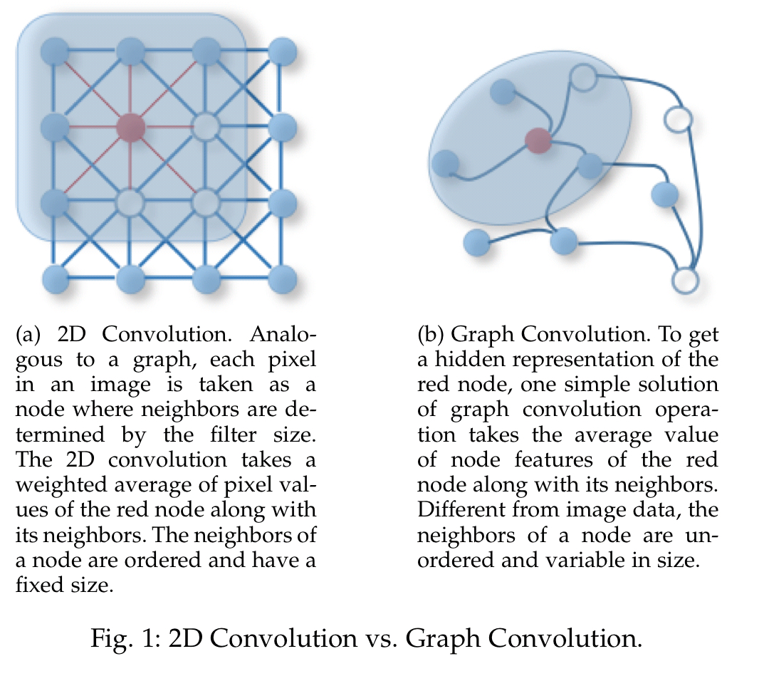
Strictly this is a spatial GCN, there are also spectral-based GCNs which interpret graphs as a signal (normalising the structure and laying the nodes out in order to form the signal). I find the spectral approach much less intuitive, but thankfully spatial models seem to be where all the action this these days.
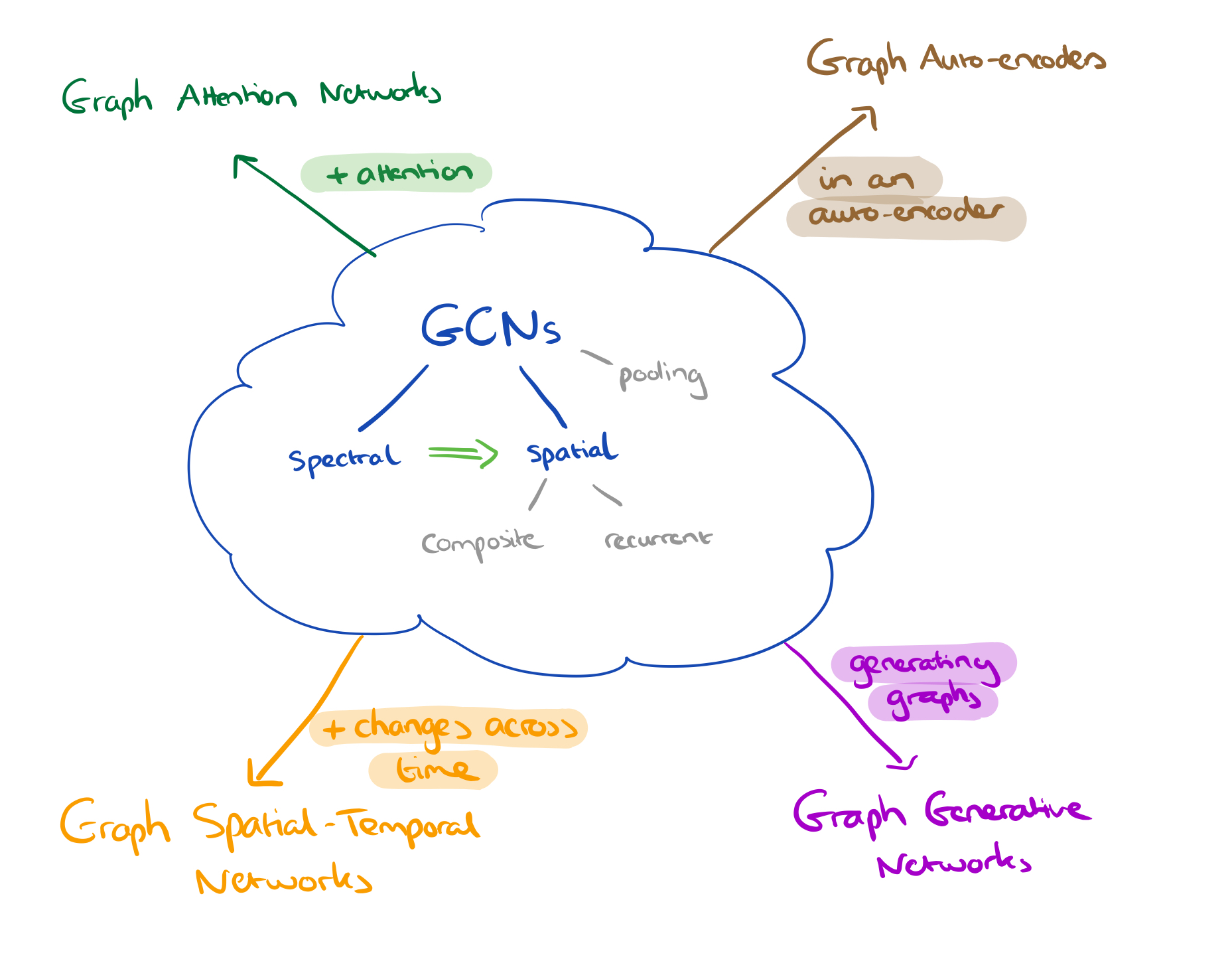
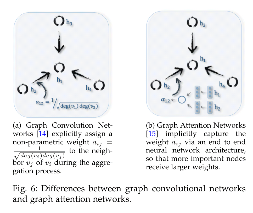
If we add the concept of attention, we arrive at Graph Attention Networks.
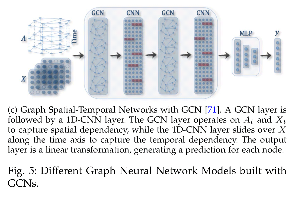
If we add the idea that the graph changes over time then we get to Graph Spatial-Temporal Networks. Graph Auto-encoders combine the familiar encoder-decoder pairs, but using graph representations on both sides. Finally, the class of Graph Generative Networks aim to generate plausible structures from data.
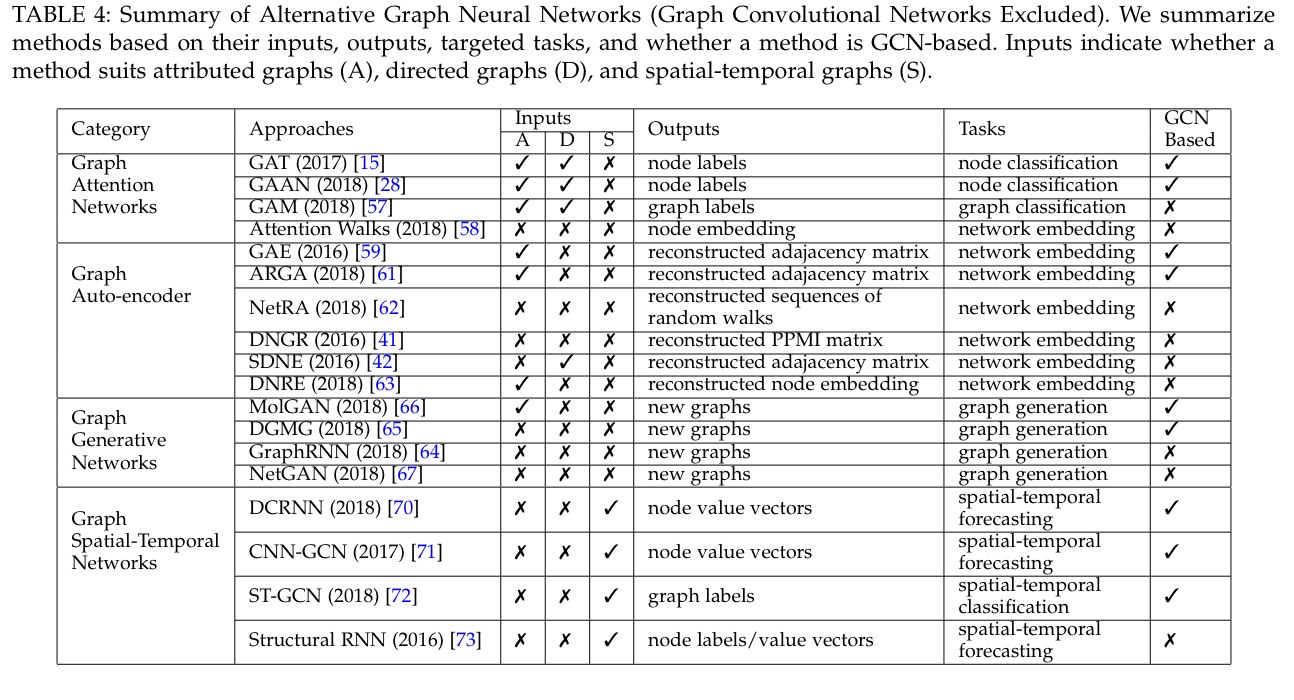
The following table highlights some of the key approaches in these extended application areas.
GCNs
The following table highlights a selection of GCN approaches.
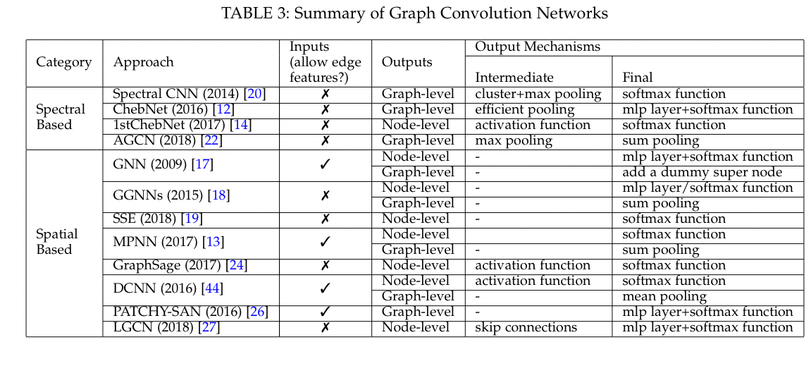
The earliest networks used a spectral approach, with graph signal filters performing convolution operations. However spectral-based models have a number of limitations: they can’t easily scale to larger graphs as the computational cost increases dramatically with graph size; they assume a fixed graph, so they generalise poorly to different graphs; and they only work on undirected graphs (§4.4). Spatial models have therefore been attracting increasing attention.
In the domain of spatial GCNs there are two further main divisions. Recurrent-based methods apply the same graph convolution layer repeatedly over time until a stable fixed point is reached. Composition-based GCNs stack a number of convolutional layers, much like a classic CNN. A representative example here is Message-Passing Neural Networks.
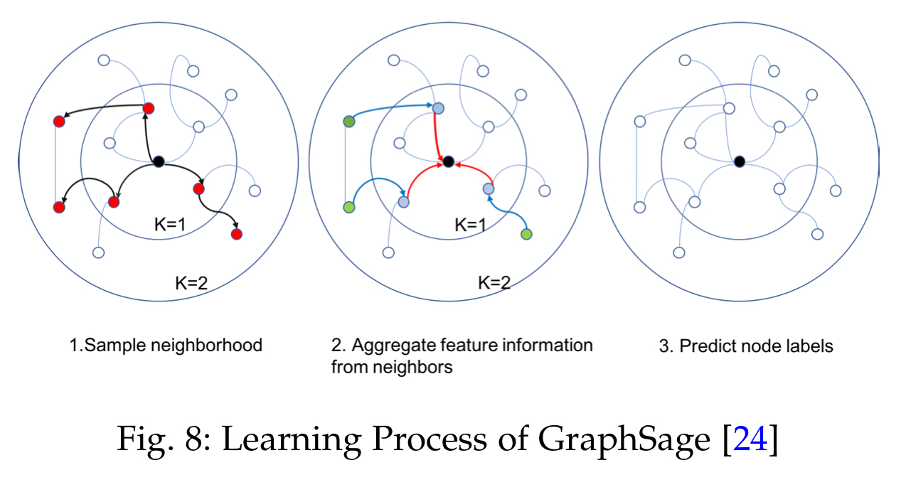
To help scale to larger graphs, GraphSage introduces a sampling batch training algorithm. It first samples the k-hop neighbourhood of a node, then derives that node’s final state by aggregating the feature information of the sampled neighbours. This derived state is then used to make predictions and backpropagate errors.
If we want to throw a few pooling layers into mix to keep things manageable, then we’ll need a way of doing graph pooling.
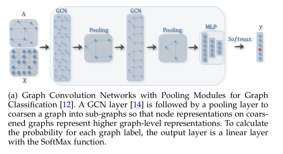
Images have a natural structure for pooling, for graphs we can use sub-graphs as the pools. DIFFPOOL provides a general solution for hierarchical pooling of nodes across a broad set of input graphs, and can be used in end-to-end training. It learns a cluster assignment matrix based on cluster node features and a coarsened adjacency matrix.
Graph Auto-encoders
Graph auto-encoders learn low dimensional node vectors via an encoder, and then reconstruct the graph via a decoder. They can be used to learn graph embeddings.
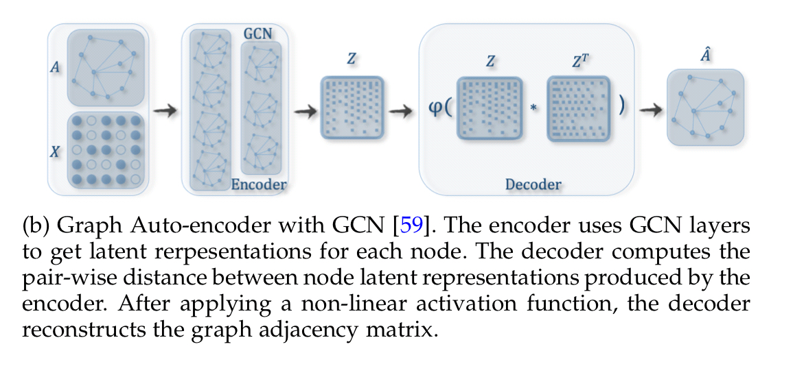
Some approaches learn node embeddings based only on topological structure, while others also make use of node content features.
Graph Spatial-Temporal networks
Graph spatial-temporal networks have a global graph structure with inputs to the nodes changing across time. For example, a traffic network (the structure) with traffic arriving over time (the content). This is modelled as Input tensors
Graph generative networks
An example in this category is MolGAN (Molecular Generative Adversarial Networks), which integrates relational GCN, improved GAN, and reinforcement learning.
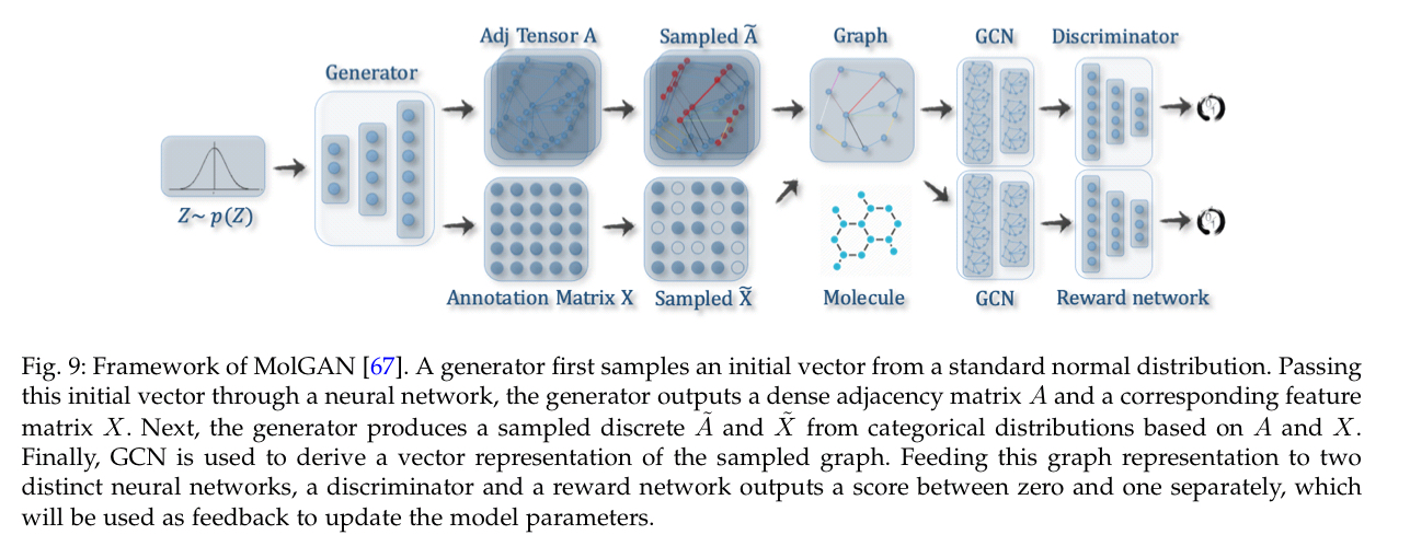
In MolGAN, the generator tries to propose a fake graph along with its feature matrix while the discriminator aims to distinguish the faked sample from the empirical data. Additionally, a reward network is introduced in parallel with the discriminator to encourage the generated graphs to possess certain properties according to an external evaluator.
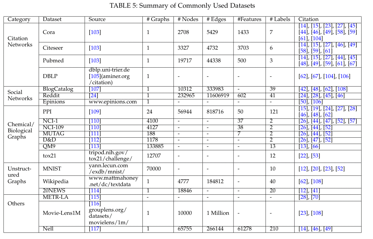
Datasets & Benchmarks
The most commonly used datasets to benchmark graph neural networks are shown in the table below.
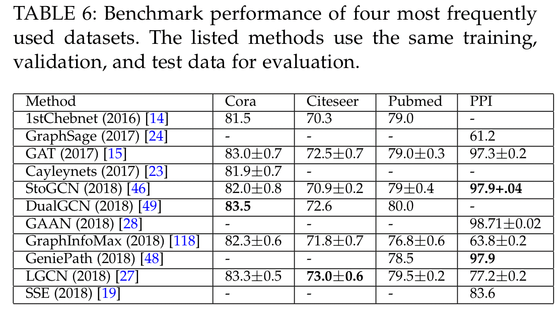
And for the four most frequently used datasets (Cora, Citeseer, Pubmed, and PPI), here are the leading models:
Research challenges and directions
I’ve only been able to scratch the surface of this 22 page survey in this short write-up. It’s clear that interest in graph neural networks is growing at a pace, but there are still a number of research challenges to be addressed.
- We haven’t figured out how to go deep with graph layers without model performance dropping off dramatically. It’s possible that depth is not a good strategy for learning graph-structured data.
- In many graphs of interest node degrees follow a power-law distribution, and hence some nodes have a huge number of neighbours and many nodes have very few. Researchers are trying to figure out how to deal with this problem through effective sampling strategies. I politely suggest they might want to look into edge partitioning too.
- Scaling to larger graphs, especially with multiple layers, remains difficult.
- Most current approaches assume static homogenous graphs. Neither of those conditions hold in many real world graphs that have different attributes for different node types, and where nodes and edges may come and go over time.

Is anybody aware of examples applying graph spatio-temporal networks to diagnostic problems, such as system diagnostics? E.g., given metric anomalies distributed over the nodes and edges in a service topology, and unfolding over time, can we classify incidents, predict future system state, identify triggering anomalies, etc.?
Good study of the space. Would love to know if you came across applications if GNN in road network other than traffic prediction problems. TIA