Graph neural networks: a review of methods and applications Zhou et al., arXiv 2019
It’s another graph neural networks survey paper today! Cue the obligatory bus joke. Clearly, this covers much of the same territory as we looked at earlier in the week, but when we’re lucky enough to get two surveys published in short succession it can add a lot to compare the two different perspectives and sense of what’s important. In particular here, Zhou et al., have a different formulation for describing the core GNN problem, and a nice approach to splitting out the various components. Rather than make this a standalone write-up, I’m going to lean heavily on the Graph neural network survey we looked at on Wednesday and try to enrich my understanding starting from there.
An abstract GNN model
For this survey, the GNN problem is framed based on the formulation in the original GNN paper, ‘The graph neural network model,’ Scarselli 2009.
Associated with each node is an s-dimensional state vector.
The target of GNN is to learn a state embedding
which contains the information of the neighbourhood for each node.
Given the state embedding we can produce a node-level output
, for example, a label.
The local transition function, 


.
Where
are the features of node
, and
are the features of its edges.
and
are the state and node features for the neighbourhood of

If we stack all the embedded states into one vector, 


, and

Where F is the global transition function and _G is the global output function.
The original GNN iterates to a fix point using 
Graph types, propagation steps, and training methods
Zhou et al. break their analysis down into three main component parts: the types of graph that a method can work with, the kind of propagation step that is used, and the training method.
Graph types
In the basic GNN, edges are bidirectional, and nodes are homogenous. Zhou et al. consider three extensions: directed graphs, heterogenous graphs, and attributed edges.
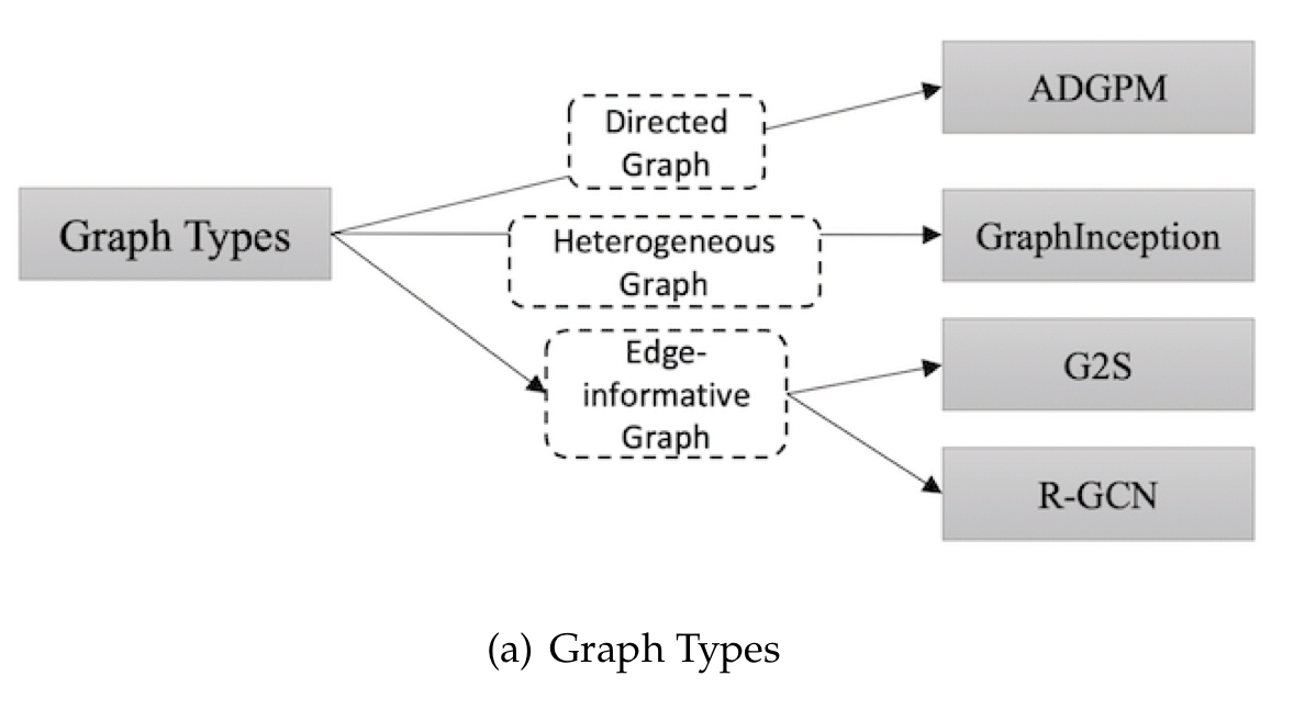
When edges have attributes there are two basic strategies: you can associate a weight matrix with the edges, or you can split the original edge into two introducing an ‘edge node’ in the middle (which then holds the edge attributes). If there are multiple different types of edges you can use one weight and one adjacency matrix per edge type.
For graphs with several different kinds of node the simplest strategy is to concatenate a one-hot encoded node type vector to the node features. GraphInception creates one neighbourhood per node type and deals with each as if it were a sub-graph in a homogenous graph.
Propagation steps
There are lots of different approaches to propagation. Many of which we looked at earlier this week .
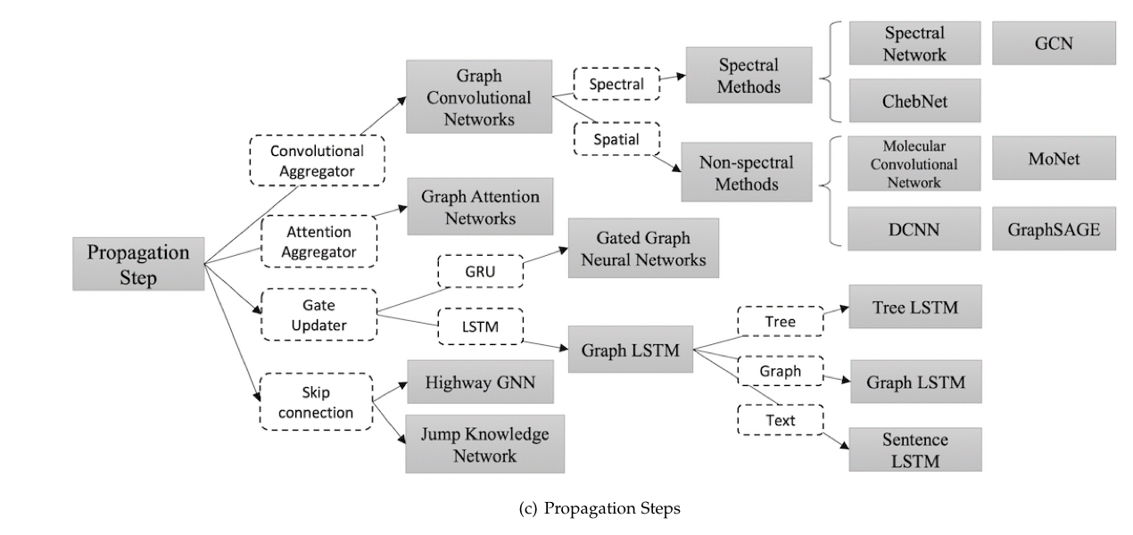
Gated approaches use Gate Recurrent Units (GRU) or LSTM models to try and improve long-term propagation of information across the graph structure. Gated Graph Neural Network (GGNN) uses GRUs with update functions that incorporate information from other nodes and from the previous timestep. Graph LSTM approaches adapt LSTM propagation based on a tree or graph. In Tree-LSTM each unit contains one forget gate and parameter matrix per child, allowing the unit to selectively incorporate per-child information. The tree approach can be generalised to an arbitrary graph, one application of which is in sentence encoding: Sentence-LSTM (S-LSTM) converts the text into a graph and then uses a Graph LSTM to learn a representation.
Another classic approach to try and improve learning across many layers is the introduction of skip connections. Highway GCN uses ‘highway gates’ which sum the output of a layer with its input and gating weights. The Jump Knowledge Network selects from amongst all the intermediate representations for each node at the last layer (the selected representation ‘jumps’ to the output layer).
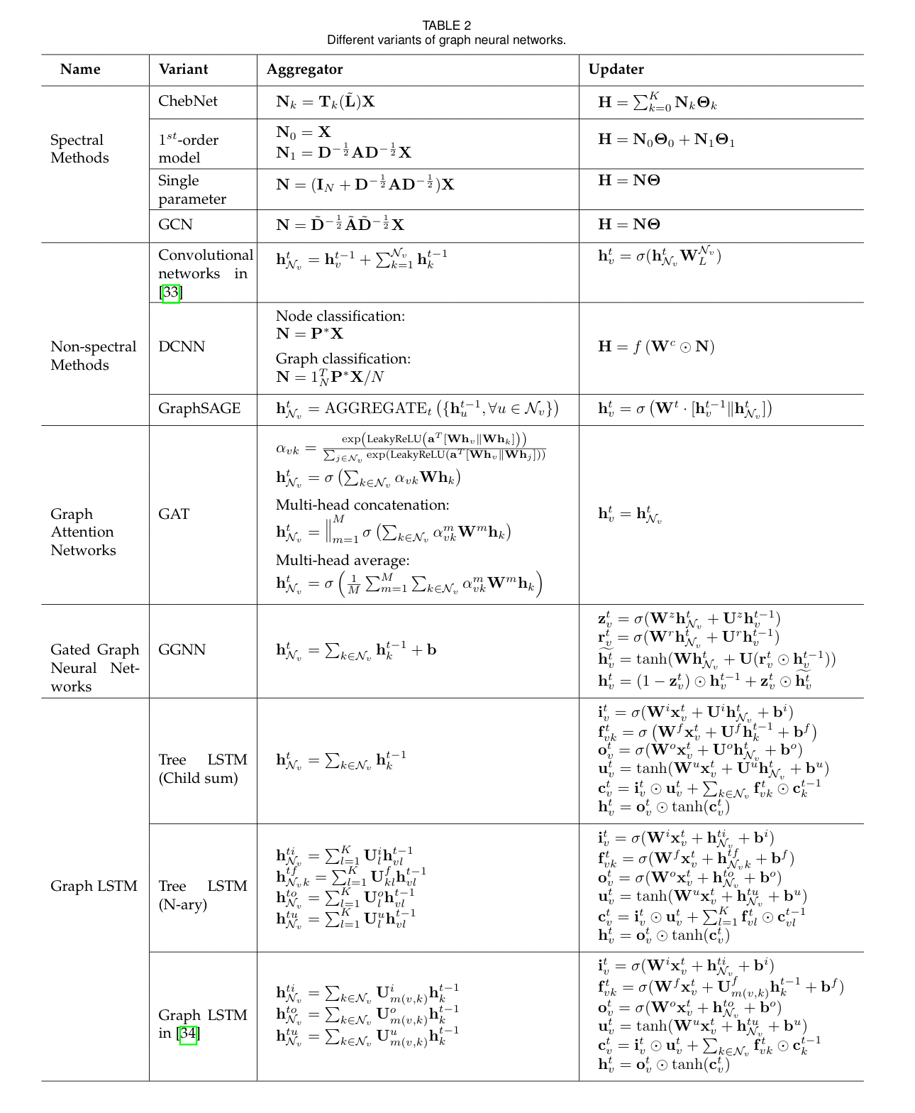
The following monster table shows how some of the different GNN methods map into the abstract model we started with.
Training methods
GNNs struggle with large graphs, so a number of training enhancements have been proposed.
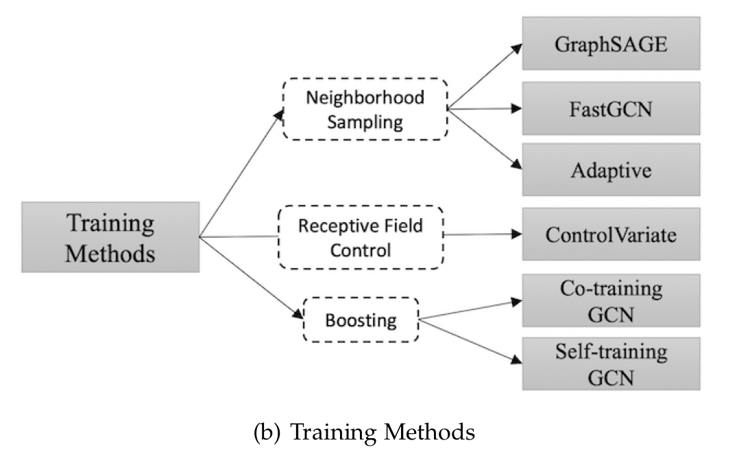
GraphSage, as we saw earlier this week, uses neighbourhood sampling. The control-variate based approach uses historical activations of nodes to limit the receptive field in the 1-hop neighbourhood (I’d need to read the referenced paper to really understand what that means here!). Co-training GCN and Self-training GCN both try to deal with performance drop-off in different ways: co-training enlarges the training data set by finding nearest neighbours, and self-training uses boosting.
The Graph Network
Section 2.3.3 in the paper discusses Graph Networks, which generalise and extend Message-Passing Neural Networks (MPNNs) and Non-Local Neural Networks (NLNNs). Graph networks support flexible representations for global, node, and edge attributes; different functions can be used within blocks; and blocks can be composed to construct complex architectures.
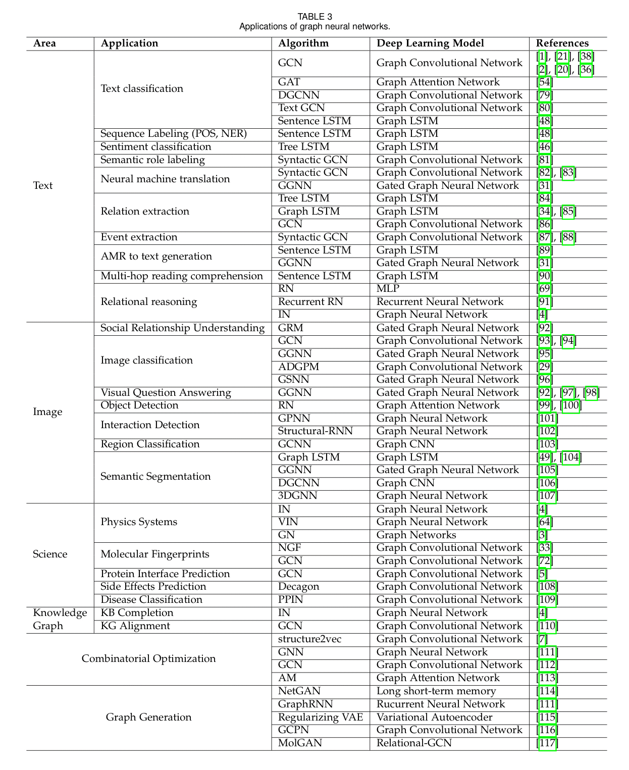
More applications of GNNs
Section 3 discusses many applications of graph neural networks, including the following handy table with references to example papers and algorithms.
Research challenges
There is good agreement on the open challenges with graph neural networks (depth, scale, skew, dynamic graphs with structure that changes over time). There’s also a discussion of the challenges involved in taking unstructured inputs and turning them into structured forms – this is a different kind of graph generation problem.
…finding the best graph generation approach will offer a wider range of fields where GNN could make a contribution.
