Gorilla: A fast, scalable, in-memory time series database – Pelkonen et al. 2015
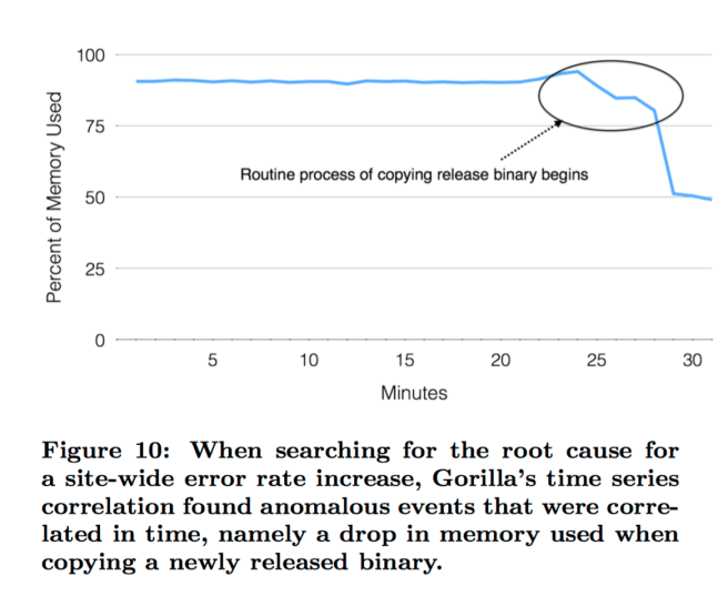
Error rates across one of Facebook’s sites were spiking. The problem had first shown up through an automated alert triggered by an in-memory time-series database called Gorilla a few minutes after the problem started. One set of engineers mitigated the immediate issue. A second group set out to find the root cause. They fired up Facebook’s time series correlation engine built on top of Gorilla, and searched for metrics showing a correlation with the errors. This showed that copying a release binary to Facebook’s web servers (a routine event) caused an anomalous drop in memory used across the site…
In the 18 months prior to publication, Gorilla helped Facebook engineers identify and debug several such production issues.
An important requirement to operating [these] large scale services is to accurately monitor the health and performance of the underlying system ad quickly identify and diagnose problems as they arise. Facebook uses a time series database to store system measuring data points and provides quick query functionalities on top.
As of Spring 2015, Facebook’s monitoring systems generated more than 2 billion unique time series of counters, with about 12 million data points added per second – over 1 trillion data points per day. Here then are the design goals for Gorilla:
- Store 2 billion unique time series, identifiable via a string key
- Insertion rate of 700 million data points (time stamp and floating point value) per minute
- Data to be retained for fast querying over the last 26 hours
- Up to 40,000 queries per second at peak
- Reads to succeed in under one millisecond
- Support time series with up to 15 second granularity (4 points/minute/time series)
- Two in-memory replicas (not co-located) for DR
- Continue to serve reads in the face of server crashes
- Support fast scans over all in-memory data
- Handle continued growth in time series data of 2x per year!
To meet the performance requirements, Gorilla is built as an in-memory TSDB that functions as a write-through cache for monitoring data ultimately written to an HBase data store. To meet the requirements to store 26 hours of data in-memory, Gorilla incorporates a new time series compression algorithm that achieves an average 12x reduction in size. The in-memory data structures allow fast and efficient scans of all data while maintaining constant time lookup of individual time series.
The key specified in the monitoring data is used to uniquely identify a time series. By sharding all monitoring data based on these unique string keys, each time series dataset can be mapped to a single Gorilla host. Thus, we can scale Gorilla by simply adding new hosts and tuning the sharding function to map new time series data to the expanded set of hosts. When Gorilla was launched to production 18 months ago, our dataset of all time series data inserted in the past 26 hours fit into 1.3TB of RAM evenly distributed across 20 machines. Since then, we have had to double the size of the clusters twice due to data growth, and are now running on 80 machines within each Gorilla cluster. This process was simple due to the share-nothing architecture and focus on horizontal scalability.
The in-memory data structure is anchored in a C++ standard library unordered map. This proved to have sufficient performance and no issues with lock contention. For persistence Gorilla stores data in GlusterFS, a POSIX-compliant distributed file system with 3x replication. “HDFS, or other distributed file systems would have sufficed just as easily.” For more details on the data structures and how Gorilla handles failures, see sections 4.3 and 4.4 in the paper. I want to focus here on the techniques Gorilla uses for time series compression to fit all of that data into memory!
Time series compression in Gorilla
Gorilla compresses data points within a time series with no additional compression used across time series. Each data point is a pair of 64-bit values representing the time stamp and value at that time. Timestamps and values are compressed separately using information about previous values.
When it comes to time stamps, a key observation is that most sources log points at fixed intervals (e.g. one point every 60 seconds). Every now and then the data point may be logged a little bit early or late (e.g., a second or two), but this window is normally constrained. We’re now entering a world where every bit counts, so if we can represent successive time stamps with very small numbers, we’re winning… Each data block is used to store two hours of data. The block header stores the starting time stamp, aligned to this two hour window. The first time stamp in the block (first entry after the start of the two hour window) is then stored as a delta from the block start time, using 14 bits. 14 bits is enough to span a bit more than 4 hours at second resolution so we know we won’t need more than that.
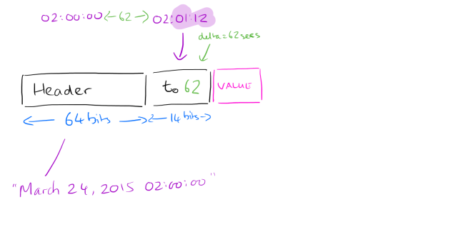
For all subsequent time stamps, we compare deltas. Suppose we have a block start time of 02:00:00, and the first time stamp is 62 seconds later at 02:01:02. The next data point is at 02:02:02, another 60 seconds later. Comparing these two deltas, the second delta (60 seconds), is 2 seconds shorter than the first one (62). So we record -2. How many bits should we use to record the -2? As few as possible ideally! We can use tag bits to tell us how many bits the actual value is encoded with. The scheme works as follows:
- Calculate the delta of deltas: D = (tn – tn-1) – (tn-1 – tn-2)
- Encode the value according to the following table:
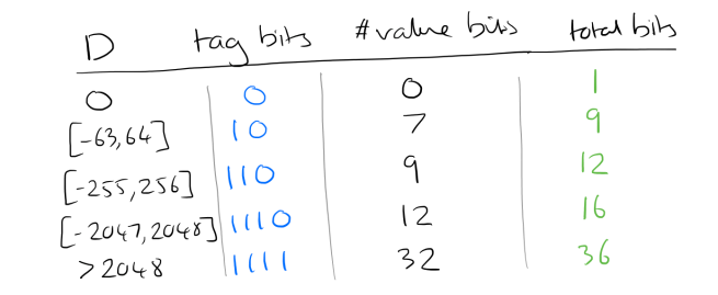
The particular values for the time ranges were selected by sampling a set of real time series from production systems and choosing the ranges that gave the best compression ratios.
This produces a data stream that looks like this:
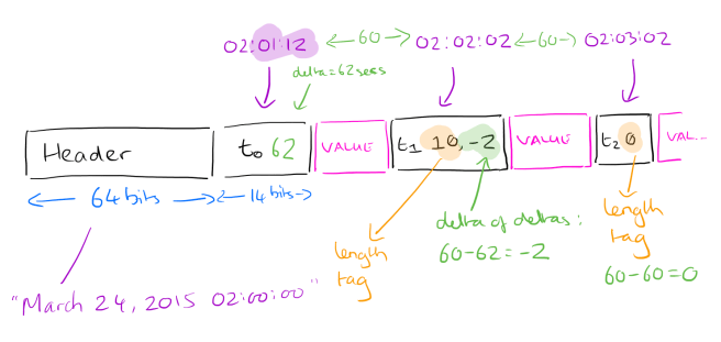
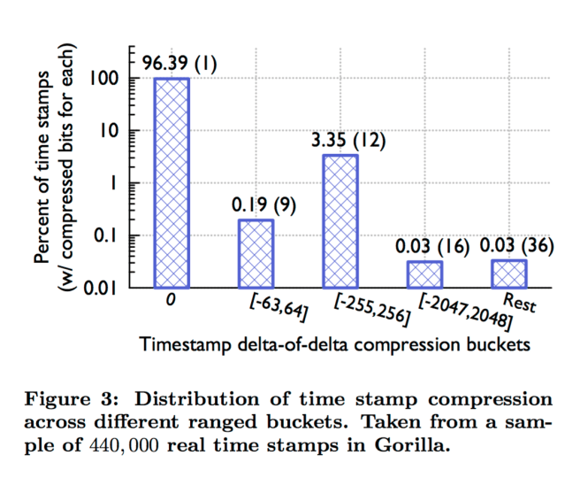
Figure 3 shows the results of time stamp compression in Gorilla. We have found that about 96% of all time stamps can be compressed to a single bit.
(i.e., 96% of all time stamps occur at regular intervals, such that the delta of deltas is zero).
So much for time stamps, what about the data values themselves?
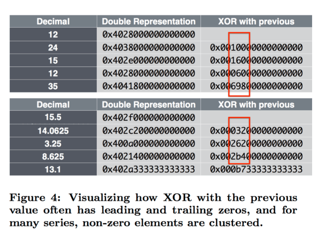
We discovered that the value in most time series does not change significantly when compared to its neighboring data points. Further, many data sources only store integers. This allowed us to tune the expensive prediction scheme in [25] to a simpler implementation that merely compares the current value to the previous value. If values are close together the sign, exponent, and first few bits of the mantissa will be identical. We leverage this to compute a simple XOR of the current and previous values rather than employing a delta encoding scheme.
The values are then encoded as follows:
- The first value is stored with no compression
- For all subsequent values, XOR with the previous value. If the XOR results in 0 (i.e. the same value), store the single bit ‘0’.
- If the XOR doesn’t result in zero, it’s still likely to have a number of leading and trailing zeros surrounding the ‘meaningful bits.’ Count the number of leading zeros and the number of trailing zeros. E.g. with 0x0003200000000000 there are 3 leading zeros and 11 trailing zeros. Store the single bit ‘1’ and then…
- If the previous stored value also had the same or fewer leading zeros, and the same or fewer trailing zeros we know that all the meaningful bits of the value we want to store fall within the meaningful bit range of the previous value:

Store the control bit ‘0’ and then store the meaningful XOR’d value (i.e. 032) in the example above.
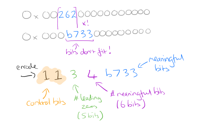
- If the meaningful bits do not fit within the meaningful bit range of the previous value, then store the control bit ‘1’ followed by the number of leading zeros in the next 5 bits, the length of the meaningful XOR’d value in the next 6 bits, and finally the meaningful bits of the XOR’d value.
Roughly 51% of all values are compressed to a single bit since the current and previous values are identical. About 30% of the values are compressed with the control bits ’10’ with an average compressed size of 26.6 bits. The remaining 19% are compressed with control bits ’11’, with an average size of 36.9 bits, due to the extra overhead required to encode the length of leading zero bits and meaningful bits.
Building on top of Gorilla
Gorillas’ low latency processing (over 70x faster than the previous system it replaced) enabled the Facebook team to build a number of tools on top, these include horizon charts; aggregated roll-ups which update based on all completed buckets every two hours; and a correlation engine that we saw being used in the opening case study.
The correlation engine calculates the Pearson Product-Moment Correlation Coefficient (PPMCC) which compares a test time series to a large set of time series. We find that PPMCC’s ability to find correlation between similarly shaped time series, regardless of scale, greatly helps automate root-cause analysis and answer the question “What happened around the time my service broke?”. We found that this approach gives satisfactory answers to our question and was simpler to implement than similarly focused approaches described in the literature[10, 18, 16]. To compute PPMCC, the test time series is distributed to each Gorilla host along with all of the time series keys. Then, each host independently calculates the top N correlated time series, ordered by the absolute value of the PPMCC compared to the needle, and returning the time series values. In the future, we hope that Gorilla enables more advanced data mining techniques on our monitoring time series data, such as those described in the literature for clustering and anomaly detection [10, 11, 16].
Summing up lessons learned the authors provide three further takeaways:
- Prioritize recent data over historical data. Why things are broken right now is a more pressing question than why they were broken 2 days ago.
- Read latency matters – without this the more advanced tools built on top would not have been practical
- High availability trumps resource efficiency.
We found that building a reliable, fault tolerant system was the most time consuming part of the project. While the team prototyped a high performance, compressed, in-memory TSDB in a very short period of time, it took several more months of hard work to make it fault tolerant. However, the advantages of fault tolerance were visible when the system successfully survived both real and simulated failures.

I would like to explore and evaluate.. I don’t find the software for download for installation.. Can you please let us know if this software is available for public to use and explore? Is it an open source?
Hi Jay, This is a Facebook internal system and as far as I know they have no plans to make it available outside their organisation. Regards, Adrian.
It’s been open-sourced now: https://github.com/facebookincubator/beringei/
From where shall I download the software for evaluation?
it seems very complicated to decompress the timestamp and value?