BTrDB: Optimizing Storage System Design for Timeseries Processing – Anderson & Culler 2016
It turns out you can accomplish quite a lot with 4,709 lines of Go code! How about a full time-series database implementation, robust enough to be run in production for a year where it stored 2.1 trillion data points, and supporting 119M queries per second (53M inserts per second) in a four-node cluster? Statistical queries over the data complete in 100-250 ms while summarizing up to 4 billion points. It’s pretty space-efficient too, with a 2.9x compression ratio. At the heart of these impressive results, is a data structure supporting a novel abstraction for time-series data: a time partitioning, copy-on-write, version-annotated, k-ary tree.
So here’s the plan. First let’s talk a little about the background motivation for the work (bonus – I got to learn what a microsynchrophasor is!), and how the requirements for an anticipated 44 quadrillion data points per year per server break existing TSDBs. Then I want to focus on the core abstraction and data structure, before finishing up with a brief look at the BTrDB system as a whole. (BTrDB btw. stands for Berkeley Tree Database, which the authors don’t actually tell you in the paper itself!).
Industrial IoT at scale – quadrillions of events per server per year
High-precision networked sensors with fairly high sample rates generate time-correlated telemetry data for electric grids, building systems, industrial processes, and so on. This data needs to be collected, distilled, and analysed both in near real-time and historically.
We focus on one such source of telemetry – microsynchrophasors, or uPMUs. These are a new generation of small, comparitively cheap and extremely high-precision power meters that are to be deployed in the distribution tier of the electrical grid, possibly in the millions… Each device produces 12 streams of 120Hz high-precision values with timestamps accurate to 100 ns (the limit of GPS).
The telemetry data also frequently arrives out of order, delayed, and duplicated. The authors set themselves a design goal of being able to support 1000 such devices per backing server. That’s about 1.4M inserts/second, and many times that in expected reads and writes from analytics.
These demands exceed the capabilities of current timeseries data stores. Popular systems such as KairosDB, OpenTSDB, or Druid, were designed for complex multi-dimensional data at low sample rates and, as such, suffer from inadequate throughput and timestamp resolution for these telemetry streams.
Cassandra exhibits the highest throughput across a number of studies, obtaining 320K inserts/sec and 220K reads/sec on a 32 node cluster.
Recently, Facebook’s in-memory Gorilla database takes a similar approach to BTrDB – simplifying the data model to improve performance. Unfortunately, it has second-precision timestamps, does not permit out-of-order insertion, and lacks accelerated aggregates. In summary, we could find no databases capable of handling 1000 uPMSs per server node (1.4 million inserts/s per node and 5x that in reads), even without considering the requirements of the analytics.
Time-partitioned trees
The key to BTrDB’s success is first of all the right abstraction designed to support the kinds of analyses anticipated for uPMU data; and secondly a highly-efficient data structure for implementing that abstraction. (The authors have great things to say about Golang too, but we’ll cover that in the next section).
The most basic operations are InsertValues – which creates a new version of a stream with the given (time,value) pairs, and GetRange which retrieves all data between two times in a given version of the stream (including the special version, ‘latest’).
BTrDB does not provide operations to resample the raw points in a stream on a particular schedule or to align raw samples across streams because performing these manipulations correctly ultimately depends on a semantic model of the data. Such operations are well supported by mathematical environments, such as Pandas…
Generally this is done as the final step after having isolated an important window – analyzing a raw stream in its entirety is impractical given that each uPMU produces nearly 50 billion samples per year!
The following access methods are far more powerful for broad analytics and for incremental generation of computationally refined streams:
- GetStatisticalRange(UUID, StartTime, EndTime, Version, Resolution) → (Version, [Time, Min, Mean, Max, Count]) retrieves statistical records between two times at a given temporal resolution.
- GetNearestValue(UUID, Time, Version, Direction) → (Version, (Time,Value)) locates the nearest point to a given time, either forwards or backwards. It is commonly used to obtain the ‘current’, or most recent to now, value of a stream of interest.
- ComputeDiff(UUID, FromVersion, ToVersion, Resolution) → [(StartTime, EndTime)] provides the time ranges that contain differences between given versions (useful to determine which input ranges have changed and hence which outputs may need to be recomputed, in the face of out of order arrival and loss).
The data structure supporting these operations is a k-ary tree.
To provide the abstraction described above, we use a time-partitioning copy-on-write version-annotated k-ary tree. As the primitives API provides queries based on time extents, the use of a tree that partitions time serves the role of an index by allowing rapid location of specific points in time. The base data points are stored in the leaves of the tree, and the depth of the tree is defined by the interval between data points. A uniformly sampled telemetry stream will have a fixed tree depth irrespective of how much data is in the tree. All trees logically represent a huge range of time (from -260 ns to 3*260 ns as measured from the Unix epoch, or approximately 1933 to 2079 with nanosecond precision) with big holes at the front and back ends and smaller holes between each of the points.
Let’s build up a tree for 16 ns of data. Here’s the starting tree that holds a list of time,value pairs for 4 ns of raw data at each leaf node.

Recall that every insert to the stream results in the creation of a new version. This is handled by labelling every link in the tree with the version that created it.
To retain historic data, the tree is copy on write: each insert into the tree forms an overlay on the previous tree accessible via a new root node. Providing historic data queries in this way ensures that all versions of the tree require equal effort to query – unlike log replay mechanisms which introduce overheads proportional to how much data has changed or how old is the version that is being queried.
Here’s an updated sketch of our tree, with the version annotations included:

A null child pointer with a nonzero version annotation implies the version is a deletion.
The time extents that were modified between two versions of the tree can be walked by loading the tree corresponding to the later version, and descending into all nodes annotated with the start version or higher. The tree need only be walked to the depth of the desired difference resolution, thus ComputeDiff returns its results without reading the raw data. This mechanism allows consumers of a stream to query and process new data, regardless of where the changes were made, without a full scan and with only 8 bytes of state maintenance required – the ‘last version processed.’
For example, if we want to ComputeDiff from version 3 to version 5 at 8 ns resolution using our sample tree we load the v 5 tree, and then simply navigate to the second level of the tree, see that the the left-hand node for t=[0,8) contains a change at v3 and v4, whereas the right-hand node does not, and return the interval list [(0,8)].
The final twist for the data structure is that each internal node also holds scalar summaries of the subtrees below it:
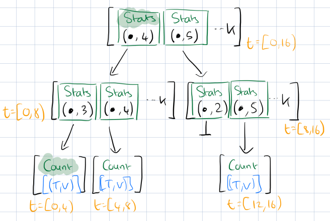
Statistical aggregates are computed as nodes are updated, following the modification or insertion of a leaf node. The statistics currently supported are min, mean, max, and count, but any operation that uses intermediate results from the child substrees without requiring iteration over the raw data can be used. Any associative operation meets this requirement.
(You can imagine a number of interesting approximate data structures being used here too).
These summaries do increase the size of internal nodes, but this represents only a tiny fraction of the total footprint. Observable statistics are guaranteed to be consistent with the underlying data, since failure during their calculation would prevent the root node from being written and hence the entire overlay would be unreachable.
When querying a stream for statistical records, the tree needs only be traversed to the depth corresponding to the desired resolution, thus the response time is proportional to the number of returned records describing the temporal extent, not the length of the extent, nor the number of data points within it.
The BTrDB implementation
The overall BTrDB system is based on a SEDA architecture.
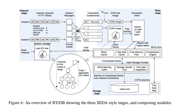
All addresses in the tree are ‘native’ and are directly resolvable by the storage layer without needing a translation step. A compression engine compresses the statistical information, address, and version fields in internal nodes, as well as the time and value fields in leaf nodes….
…it uses a method we call delta-delta coding followed by Huffman coding using a fixed tree. Typical delta coding works by calculating the difference between every value in the sequence and storing that using variable-length symbols (as the delta is normally smaller than the absolute values). Unfortunately, with high-precision sensor data, this process does not work well because nanosecond timestamps produce very large deltas, and even linearly-changing values produce sequences of large, but similar, delta values…. Delta-delta compression replaces run-length encoding and encodes each delta as the difference from the mean of a window of previous delta values. The result is a sequence of jitter values.
This technique helps to achieve a 2.9x compression ratio.
There are of course many more implementation details in the paper. This paragraph on how well matched Go is to SEDA architectures caught my eye:
SEDA advocates constructing reliable, high-performance systems via decomposition into independent stages separated by queues with admission control. Although not explicitly referencing this paradigm, Go encourages the partitioning of complex systems into logical units of concurrency, connected by channels, a Go primitive roughly equal to a FIFO with atomic enqueue and dequeue operations. In addition, Goroutines – an extremely lightweight thread-like primitive with userland scheduling – allow for components of the system to be allocated pools of goroutines to handle events on the channels connecting a system in much the same way that SEDA advocates event dispatch. Unlike SEDA’s Java implementation, however, Go is actively maintained, runs at near native speeds and can elegantly manipulate binary data.
Using Ceph as the underlying store, BTrDB achieves a third-quartile write latency at maximum load (53 million points per second for a four-node cluster) of 35ms, which is less than one standard deviation from the raw pool’s latency. See the full paper for a detailed analysis of BTrDBs performance.
The principles underlying this database are potentially applicable to a wide range of telemetry timeseries, and with slight modification, are applicable to all timeseries for which statistical aggregate functions exist and which are indexed by time.

Awesome review! Thank you!