Towards Parameter-Free Data Mining – Keogh et al. SIGKDD 2004

Another time series paper today from the Facebook Gorilla references. Keogh et al. describe an incredibly simple and easy to implement scheme that does surprisingly well with clustering, anomaly detection, and classification tasks over time series data. As per the title of the paper, it does not require any parameter tuning, and is robust to overfitting.

Everything hinges on comparing the size of compressed data! The theory behind why this works as well as it does is very elegant.

From Kolmogorov complexity to compression-based dissimilarity

The Kolmogorov complexity K(x) of a string x is defined as the length of the shortest program capable of producing x on a universal computer – such as a Turing machine…. Intuitively, K(x) is the minimal quantity of information required to generated x by an algorithm.

Let K(x|y) be the length of the shortest program that computes x given y as input, and K(xy) be the length of the shortest program that outputs y concatenated to x.

We can now consider the distance between two string as:

d_k = (K(x|y) + K(y|x)) / K(xy)

This is all well and good, but how do you compute Kolmogorov complexity?

It is easy to realize that universal compression algorithms give an upper bound to the Kolmogorov complexity. In fact, K(x) is the best compression that one could possibly achieve for the text string x. Given a data compression algorithm, we define C(x) as the size of the compressed size of x and C(x|y) as the compression achieved by first training the compression on y, and then compressing x. For example, if the compressor is based on a textual substitution method, one could build the dictionary on y, and then use that dictionary to compress x. We can approximate (1) by the following distance measure :

d_c(x,y) = (C(x|y) + C(y|x)) / C(xy)

The better the compression algorithm, the better the approximation of d_c for d_k is.

This leads us to a compression-based dissimilarity (CDM) measure:

CDM(x,y) = C(xy) / (C(x) + C(y))

The CDM dissimilarity is close to 1 when x and y are not related, and smaller than one if x and y are related. The smaller the CDM(x,y), the more closely related x and y are. Note that CDM(x,x) is not zero.

This dissimilarity measure can be very easily implemented. Some care needs to be taken with data formats to avoid artificially high compression. The example given in the data is 8-digit precision samples that have been converted to 16-bit format and hence all contain lots of zeros give false impression of similarity.

A simple solution to the problem noted above is to convert the data into a discrete format, with a small alphabet size. In this case, every part of the representation contributes about the same amount of information about the shape of the time series…. In this work we use the SAX (Symbolic Aggregate ApproXimation) representation of Lin et al. This representation has been shown to produce competitive results for classifying and clustering time series, which suggests that it preserves meaningful information from the orginal data. While SAX does allow parameters, for all experiments here we use the parameterless version.

Using CDM for clustering

Since CDM is a dissimilarity measure, it can be used directly in most standard clustering algorithms.

For some partitional algorithms, it is necessary to define the concept of cluster “center”. While we believe we can achieve this by extending the definition of CDM, or embedding it into a metric space, for simplicity here, we well confine our attention to hierarchical clustering.

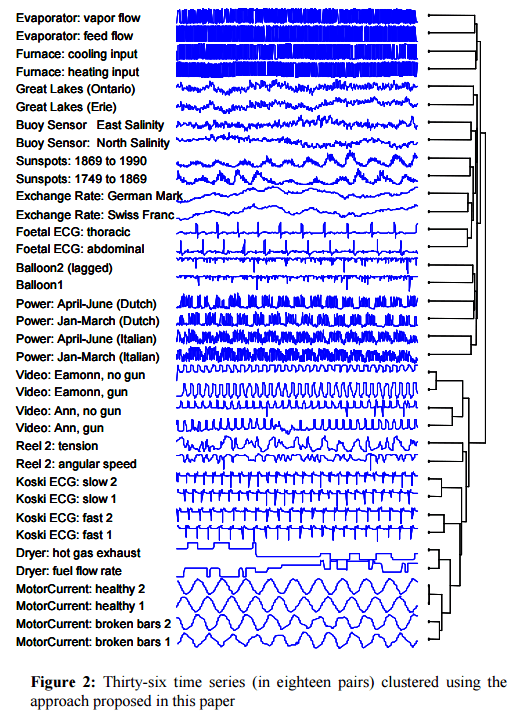
Keogh et al. tested CDM against every time series distance/dissimilarity/similarity measured that has appeared in the last decade in any of the following conferences: SIGKDD, SIGMOD, ICDM, ICDE, VLDB, ICML, SSDB, PKDD, and PAKDD – 51 in total! In addition they also considered Euclidean distance, Dynamic Time Warping, L₁, L_inf, and the Longest Commons Subsequence (LCSS). The test was done with the URC time series archive for datasets that come in pairs. A top score in this test would correctly cluster all 18 pairs in the dataset with a single bifurcation separating each pair, which CDM does. More than 3/4 of the other approaches tested did not get any of the pairs correct, the next best approaches (DTW, LCSS, HMM with SAX ) got only 1/3 correct.

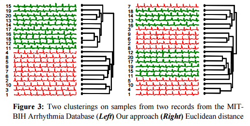
In a comparison of ECG samples, CDM again provided a much better clustering than the next-best method (Euclidean distance in this case).

CDM was also applied to clustering text – in this case DNA strings.

We took the first 16,300 symbols from the mitochondrial DNA of twelve primates and one ‘outlier’ species and hierarchically clustered them… To validate our results, we showed the resulting dendogram to an expert in primate evolution, Dr Sang-Hee Lee of UCR. Dr. Lee noted that some of the relevant taxonomy is still the subject of controversy, but informed us that the “topography of the tree looks correct.”

Using CDM for anomaly detection

To detect anomalies in time series with CDM, the authors propose a simple divide-and-conquer algorithm:

Both the left and the right halves of the entire sequence being examined are compared to the entire sequence using the CDM dissimilarity measure. The intuition is that the side containing the most unusual section will be less similar to the global sequence than the other half. Having identified the most interesting side, we can recursively repeat the above, repeatedly dividing the most interesting section until we can no longer divide the sequence.

This technique outperformed four state-of-the-art (2004) algorithms on a wide variety of real and synthetic problems. It is further improved by using the SAX representation when working with the time series. As described above, it assumes a single anomaly in the dataset, and also that – especially in the first few iterations – it can detect the difference a small anamoly makes even when surrounded by a large amount of normal data.

A simple solution to these problems is to set a parameter W, for number of windows. We can divide the input sequence into W contiguous sections, and assign the anomaly value of the i^th window as CDM(W_i, data ). In other words, we simply measure how well a small local section can match the global sequence. Setting this parameter is not too burdensome for many problems. For example of the ECG dataset discussed in Section 4.2.3, we found that we could find the objectively correct answer, if the size of the window ranged anywhere from a ¼ heartbeat length to four heartbeats. For clarity, we call this slight variation Window Comparison Anomaly Detection (WCAD).

In the ‘noisy sine’ test CDM easily finds the anomaly (thick line, row A). SVM (row B) finds it with careful parameter tuning, and IMM, which is stochastic, finds it in most runs. CDM is orders of magnitude faster though, and does not require setting any parameters.

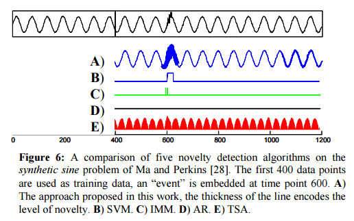
Testing against a variety of datasets, the authors found that both SVM and IMM could be tuned to find the anamoly on any individual sequence, but once the parameters were so tuned they did not generalize to the other problems.

The objective of these experiments is to reinforce the main point of this work. Given the large number of parameters to fit, it is nearly impossible to avoid overfitting.

On the MIT-BIH noise stress test database, CDM found the same two anomalies that a cardiologist independently annotated. “All the other approaches produced results that were objectively (per the cardiolgists’ annotations) and subjectively incorrect, in spite of careful parameter tuning.”

The technique can be applied to multi-dimensional time series by collecting the results on each individual dimension and then linearly combining them into a single measure of novelty.

Using CDM for classification

Because CDM is a dissimilarity measure, we can trivially use it with a lazy-learning scheme. For simplicity, in this work, we will only consider the one-nearest-neighbor algorithm.

CDM was compared against Dynamic Time Warping (DTW) and Euclidean Distance on ECG datasets (four patients), and on a video dataset of actors performing various actions with guns (2 actors, both with and without guns). There are two ECG signal series, and the task is to classify points by patient from a time series with instances extracted from all four patients. In the gun data set there is a two-class classification problem to identify actor A vs actor B, and a four-class classification problem identifying A-with-gun, A-without-gun, B-with-gun, and B-without-gun.

Here’s how CDM performed:

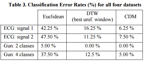
In all four datasets discussed above, Euclidean distance is extremely fast, yet innaccurate. DTW with the best uniform window size greatly reduces the error rates but took several orders of magnitude longer. However, CDM outperforms both Euclidean and DTW in all datasets. Even though CDM is slower than Euclidean distance, it is much faster than the highly optimized DTW.