Finding Surprising Patterns in a Time Series Database in Linear Time and Space – Keogh et al. SIGKDD 2002

In the Facebook Gorilla paper, the authors mentioned a number of additional time series analysis techniques they’d like to add to the system over time. Today’s paper is one of them, and it deals with the question of how to find surprising or anomalous patterns within a time series dataset.

Note that this problem should not be confused with the relatively simple problem of outlier detection. Hawkins’ classic definition of an outlier is “… an observation that deviates so much from other observations as to arouse suspicion that it was generated from a different mechanism.” However, we are not interested in finding individually surprising datapoints, we are interesting in finding surprising patterns, i.e. combinations of data points whose structure and frequency somehow defies our expectations.

A pattern is defined as surprising if the frequency of its occurrence differs substantially from that expected by chance, given some previously seen data. Thus there is no need to somehow specify what to ‘look for’ that might constitute a surprise. The only pre-requisite is availability of data considered to be normal (non-surprising).

A time series pattern P, extracted from database X is surprising relative to a database R, if the frequency of its occurrence is greatly different to that expected by chance, assuming that R and X are created by the same underlying process.

The high-level steps of the Tarzan algorithm are as follows:

• First turn the input time series X into a discretized time series over some fixed size set of tokens a (the alphabet). (This will later allow us to compute the probability of an occurrence, avoiding the paradox that the probability of a particular real number being chosen from any distribution is zero).
• Do the same thing with the reference time series R
• Create suffix trees for the discretized time series of X and R, and use a Markov model to determine how likely the substrings represented by the nodes in the suffix tree of X are.
• Move a sliding window over the discretized time series for X, and look-up the surprise score for each window using the pre-calculated scores in the previous step.
• Flag as surprising any window with a score over some threshold.

We’ll look at the details of discretizing the time series, computing the suffix trees, and determining likelihood shortly.

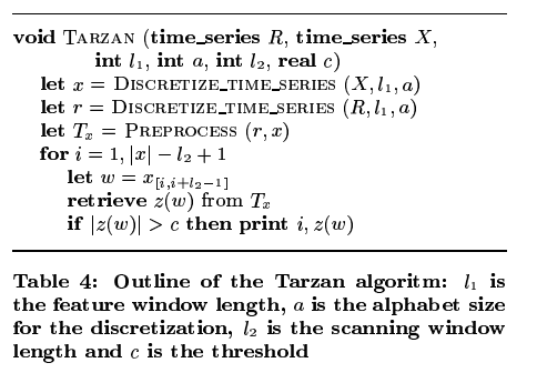
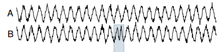
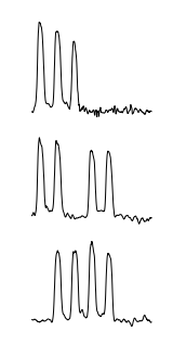
As an example of Tarzan at work, consider a noisy sine wave as the reference time series (A in the illustration below), and a synthetic anomaly introduced as a test (B in the illustration below – in which the period of the time series is temporarily halved). Tarzan shows a strong ‘suprise’ peak for the duration of the anamoly (E).

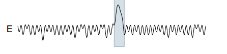
Tarzan was also tested on a real world power demand dataset for a Dutch research facility. The reference pattern shows strong peaks for weekdays, followed by relatively quiet weekends:

The three most surprising weeks in the dataset as found by Tarzan are illustrated below:

Tarzan returned three sequences that correspond to the weeks that contain national holidays in the Netherlands. In particular, from top to bottom, the week spanning both December 25th and 26th and the weeks containing Wednesday April 30th (Koninginnedag, “Queen’s Day”) and May 19th (Whit Monday) respectively.

When tested with truly random data, after seeing enough of it, Tarzan found any ‘patterns’ to be less and less surprising (i.e. Tarzan doesn’t generate false positive surprises).

Let’s build back up to a complete understanding of how Tarzan works.

Discretizing time series

In order to compute this (surprise) measure, we must calculate the probability of occurrence for the pattern of interest. Here we encounter the familiar paradox that the probability of a particular real number being chosen from any distribution is zero. Since a time series is an ordered list of real numbers the paradox clearly applies. The obvious solution to this problem is to discretize the time series into some finite alphabet Σ. Using a finite alphabet allows us to avail of Markov models to estimate the expected probability of occurrence of a previously unseen pattern.

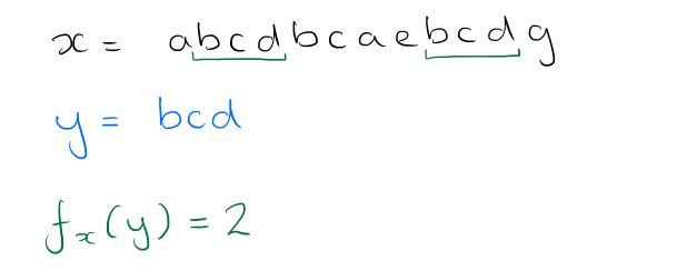
What we want to end up with is a string (ordered sequence) of symbols from the alphabet Σ. If a string x can be decomposed into the sequence uvw where u, v and w are substrings (or words) of x, then u is called a prefix of x, and w is called a suffix. A string y has an occurrence at position i of some text x if the substring of x starting at position i, of length |y|, is equal to y. The authors use f_x(y) to denote the number of occurrences of y in x.

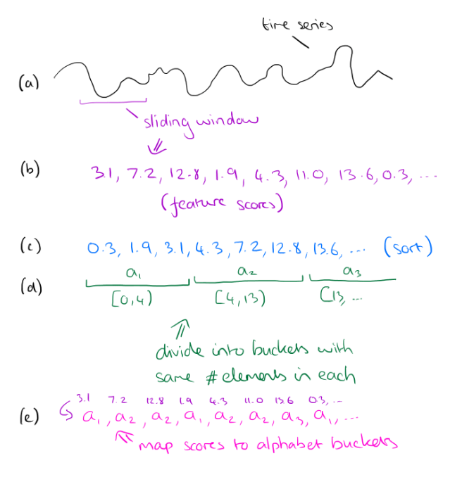
To discretize the stream, choose an alphabet size and a feature window length. Slide the feature window over the time series, and at each step examine the data within the window and compute a single real number from it. This real number should be computed so as to represent some feature of the data (you can use any function that makes sense in your domain, in the paper, the authors use the slope of the best-fitting line).

Take all of the computed scores and sort them. Based on this sorted list, derive alphabet size buckets such that an equal number of scores falls within each bucket. Now go back over the sequence of scores, and replace each score by number of the bucket that it falls into. The whole process is illustrated below:

For large databases the feature boundaries will be very stable, and so instead of sorting the entire dataset it is possible to take a subsample and compute the buckets based on that instead. If the subsample is of size √|R| then the feature extraction algorithm is O(R).

Building a suffix tree

A space efficient structure to count the number of occurrences of each substring in a sequence is a suffix tree. (We need those counts to figure out how surprising they are in the next step of the Tarzan algorithm…).

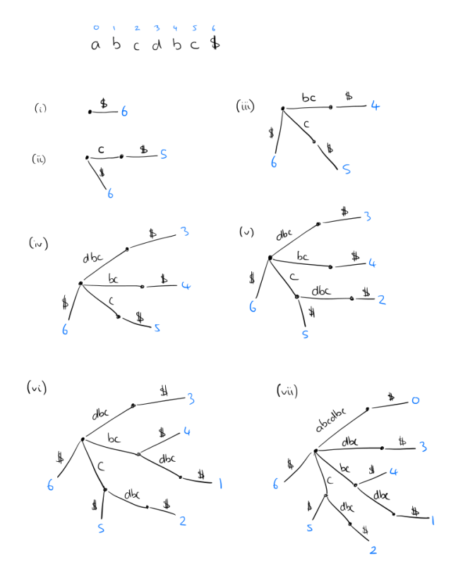
For a string of length n, a suffix tree has n leaves, numbered 1 to n, following a path through the tree from the root to leaf number i gives the suffix that begins at index i in the string. It’s easiest to understand the constructing by reversing the string and building the tree up from there as in the sketch below. But several clever constructions are available with O(n log|Σ|), as well as linear time on-line algorithms (i.e., proceeding character by character through the string from first to last).

The whole tree can be stored in linear space by keeping index pointers to occurences of the labels in the text rather than storing the labels themselves.

Having built the tree, some additional processing makes it possible to count and locate all the distinct instances of any pattern in O(m) time, where m is the length of the pattern…

Suppose we want to find and count all instances of a word w (e.g. ‘bc’ in the example above). Find the locus node __ in the tree that represents w, or the shortest extension of w if w ends in the middle of an arc. The number of occurrences f_x(w) is given by the number of the leaves in the subtree rooted at __.

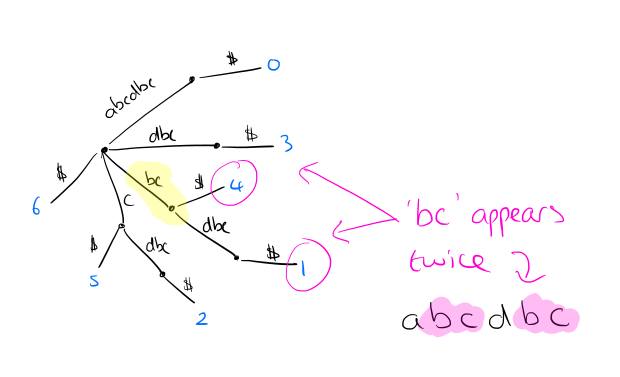
We can process the tree and store in each internal node the number of leaves below it, making subsequent frequency lookup fast.

Computing likelihood with Markov models

Consider that a string is generated by a stationary Markov chain of order M ≥ 1 on the finite alphabet Σ. If x = x_[1],x_[2],…x_[n] is an observation of the random process, and y = y_[1],y_[2],…y_[m] is an arbitrary but fixed pattern over Σ with m < n, then the stationary Markov chain is completely determined by its transition matrix Π with transition probabilities π(y_[1,M],c).

π(y_[1,M],c) = P(X_i+1 = c | X_{[i-M+1,i] = y}[1,M])

(informally, given the sequence seen so far, what’s the probability the next character is c).

We don’t know the true Markov model that generated the string of course, but we can estimated it from an observed sequence x. In particular, the transition probability can be estimated by the maximum likelihood estimator:

π(y_[1,M],c) = f_x(y_[1,M]c) / f_x(y_[1,M]).

For example, given the string ‘abcabcabd’ we want to know the transition probability for (‘ab’,c). This is the number of occurrences of ‘abc’ (2), divided by the number of occurrences of ‘ab’ (3) – so we estimate it as 2/3.

The stationary probability is estimated by _f_x(y_[1,M]) / (n – M + 1). Returning to the ‘abcabcadb’ example, the stationary probability of ‘abc’ is 2 / (9 – 3 + 1) = 2/7.

The frequency counts needed to estimate these probabilities are handily encoded in the suffix trees. Now we are ready to estimate the likelihood of seeing the strings that we see in X, as compared to the reference series R.

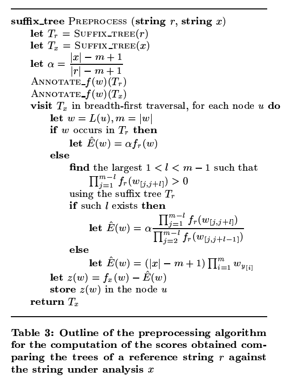
Let the scale factor α = (|x| – m + 1) / (|r| – m + 1) (i.e. the relative sizes of the sequences X and R).

Given a suffix tree T_r, built for the reference time series R, and a suffix tree T_<x built from the observed time series X, perform a breadth-first traversal of T_x examining each node u in T_x in turn.

• Compute the string w formed by traversing T_x from the root to the node u.
• Lookup w in T_r.
  • If w exists in T_r then let the expected number of occurrences of w in X be αf_r( w ) (i.e. the count that we stored at that node in T_r during preprocessing, scaled by the factor α)
  • If w doesn’t exist in T_r then find the largest l such that all substrings of length l in w exist in T_r. Set the expected number of occurrences of w in X to be

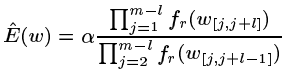
(see the full paper for the derivation of this formula)

• If there is no suitable l, set the expected number of occurrences of w in X based on the probability of the symbols from T_r
  • Set the surprise score to be the difference between the observed number of occurrences and the expected number of occurrences.

Here’s the full preprocessing algorithm: