DBSherlock: A performance diagnostic tool for transactional databases Yoon et al. SIGMOD ’16
…tens of thousands of concurrent transactions competing for the same resources (e.g. CPU, disk I/O, memory) can create highly non-linear and counter-intuitive effects on database performance.
If you’re a DBA responsible for figuring out what’s going on, this presents quite a challenge. You might be awash in stats and graphs (MySQL maintains 260 statistics and variables for example), but still sorely lacking the big picture… “as a consquence, highly-skilled and highly-paid DBAs (a scarce resource themselves) spend many hours diagnosing performance problems through different conjectures and manually inspecting various queries and log files, until the root cause is found.”
DBSherlock (available at http://dbseer.org) is a performance explanation framework that helps DBAs diagnose performance problems in a more principled manner. The core of the idea is to compare a region of interest (an anomaly) with normal behaviour by analyzing past statistics, to try and find the most likely causes of the anomaly. The result of this analysis is one or both of:
- A set of concise predicates describing the combination of system configurations or workload characteristics causing the performance anomaly. For example, when explaining an anomaly caused by a network slowdown:
network_send < 10KB
 ∧ network_recv < 10KB
 ∧ client_wait_times > 100ms
 ∧ cpu_usage < 5
- A high-level diagnosis based on existing causal models in the system. An example cause presented here might be “Rotation of the redo log file.”
Suppose in the first of these two cases the predicates are presented to the user, who diagnoses the root cause as a network slowdown based on these hints. This information is fed back to DBSherlock by accepting the predicates and labelling them with the actual cause.
This ‘cause’ and its corresponding predicates comprise a causal model, which will be utilized by Sherlock for future diagnoses.
There are a number of similarities here to works on time series discretization, anomaly detection, and correlation, but the emphasis in this work is on explaining anomalies (largely assumed to be already detected by the user because they’re of the obvious ‘performance is terrible’ kind, though automated anomaly detection can be integrated with the system) rather than detecting them.
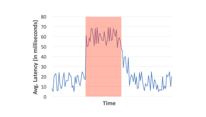
The starting point is a graph like the following, where the user can highlight a region and ask “what’s going on here?”
There are three main layers to answering that question inside DBSherlock: firstly, predicate generation seeks to find a small number of predicates that have high separation power to divide the anomalous and normal region behaviours; secondly, the set of predicates can be further pruned using simple rules encoding limited domain knowledge; and finally the causal model layer seeks to learn and map sets of predicates to higher-level causes, capturing the knowledge and experience of the DBA over time.
DBSherlock is integrated as a module in DBSeer, an open-source suite of database administration tools for monitoring and predicting database performance. This means DBSherlock can rely on DBSeer’s API for collecting and visualizising performance statistics. At one-second intervals, the following data is collected:
- OS resource consumption statistics
- DBMS workload statistics
- Timestamped query logs
- Configuration parameters from the OS and DBMS
From the raw data, DBSeer computes aggregate statistics about transactions executed during each time interval, and aligns them with the OS and DBMS statistics according to their timestamps. It is these resulting time series that DBSherlock using as the starting point for diagnosis.
Finding predicates of interest
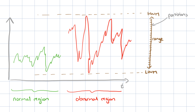
Starting from a given abnormal region, and a normal region, the aim is to find predicates that can separate them as cleanly as possible. The separation power of a predicate is defined as the difference between percentage of abnormal tuples that satisfy it, and the percentage of normal tuples that satisfy it.
Identifying predicates with high separation power is challenging. First, one cannot find a predicate of high separation power by simply comparing the values of an attribute in the raw dataset.This is because real-world datasets and OS logs are noisy and attribute values often fluctuate regardless of the anomaly. Second, due to human error, users may not specify the boundaries of the abnormal regions with perfect precision. The user may also overlook smaller areas of anomaly, misleading DBSherlock to treat them as normal regions. These sources of error compound the problem of noisy datasets. Third, one cannot easily conclude that predicates with high separation power are the actual cause of an anomaly. They may simply be correlated with, or be symptoms themselves of the anomaly, and hence, lead to incorrect diagnoses.
The first step is to discretize the time series (or each attribute within a multi-dimensional time series, if you prefer to think of it that way) within the ranges of interest. For numeric attributes, the maximum and minimum values within the ranges of interest are found, and the resulting range is divided into R equal sized buckets or partitions. For example, with a range 0–100 and R = 5 these would be [0,20), [20,40), [40,60), [60,80), and [80,100). By default DBSherlock uses R = 1000. For categorical attributes, one partition is created for each unique attribute value found. The result of this step is a partition space. (Why not use a standard time series algorithm such as SAX for this step? )
The next step is to label the partitions. For each partition, all the tuples that fall within that partition are examined. If all of these tuples are from the abnormal region, the partition is labeled as abnormal. If all of the the tuples are instead from the normal region, then the partition is labeled as normal. Otherwise it is left empty (unlabeled).
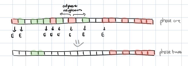
At this stage, due to the noise in the data, there will probably be a mixed set of abnormal and normal partitions such as this:

To cope with this noise, a filtering and filling process now takes place. Filtering helps to find a sharper edge separating normal and abnormal. This is a two-phase process. In the first phase each non-empty (i.e. marked as abnormal or normal) partition is examined. If it’s nearest non-empty partition in either direction is not of the same type (e.g. an abnormal partition has a normal partition as its first non-empty neighbour) then that partition is marked. In the second phase, all marked partitions are switched to empty.
Our filtering strategy aims to separate the Normal and Abnormal partitions that are originally mixed across the partition space (e.g., due to the noise in the data or user errors). If there is a predicate on attribute Attr, that has high separation power, the Normal and Abnormal partitions are very likely to form well-separated clusters after the filtering step. This step mitigates some of the negative effects of noisy data or user’s error, which could otherwise exclude a predicate with high separation power from the output.
After filtering, we will be left with larger blocks of consecutive normal and abnormal partitions, separated by empty partitions. The empty partitions are now filled by marking them as either normal or abnormal:
- If the nearest adjacent partitions to an empty partition both have the same type (e.g. abnormal), then the partition is assigned that type.
- If the nearest adjacent partitions have different types, then the partition is assigned the label of the closer partition. The distance calculation includes an anomaly distance multiplier factor δ by which the distance to an abnormal adjacent neighbour is multiplied before doing the comparison. If δ > 1 of course, this favours marking a partition as normal. DBSherlock uses δ = 10 by default.

Finally it comes time to extract a candidate predicate for the attribute. A candidate predicate is generated for a numeric attribute if the following two conditions hold:
- There is a single block of abnormal partitions
- After normalizing the attribute values so that they all fall on a spectrum from 0..1, the average value of the attribute in the normal range and the average value of the attribute in the abnormal range are separated by at least θ, where θ is a configurable normalized difference threshold.
If a numeric attribute passes these two tests, a predicate with one of the following forms will be generated:
- attr < x
- attr > x
- x < attr < y
Categorical attribute predicates are simpler, and DBSherlock simply generates the predicate Attr ∈ {p | p.label = abnormal}.
Incorporating domain knowledge
Our algorithm extracts predicates that have a high diagnostic power. However, some of these predicates may be secondary symptoms of the root cause, which if removed, can make the diagnosis even easier.
The secondary symptom predicates can be pruned with a small amount of domain knowledge. This knowledge is expressed as a set of rules of the form Attri → Attrj with the meaning that if predicates for both Attri and Attrj are generated, then the predicate for Attrj is likely to be a secondary symptom. Cycles are not allowed in the rule set.
As an example, for MySQL on Linux, there are just four rules:
- DBMS CPU Usage → OS CPU Usage. (if DBMS CPU Usage is high, we probably don’t need to also flag OS CPU Usage)
- OS Allocated Pages → OS Free Pages; OS Used Swap Space → OS Free Swap Space; OS CPU Usage → OS CPU Idle. (For these three, one attribute is always completely determined by the other, and so is uninteresting).
Causal models
Previous work on performance explanation has only focused on generating explanations in the form of predicates. DBSherlock improves on this functionality by generating substantially more accurate predicates (20–55% higher F1-measure;). However, a primary objective of DBSherlock is to go beyond raw predicates, and offer explanations that are more human-readable and descriptive.
Suppose DBSherlock finds three predicates with high predictive power for an anomaly, and after investigation the user confirms with the help of these clues that the true cause was rotation of the redo log file. “Rotation of the redo log file” is then added to the system as a causal model and linked with these three predicates.
After that, for every diagnosis inquiry in the future, DBSherlock calculates the confidence of this causal model and ‘Log Rotation’ is reported as a possible cause if its confidence is higher than a threshold λ. By default, DBSherlock displays only those causes whose confidence is higher than λ=20%. However, the user can modify λ as a knob (i.e., using a sliding bar) to interactively view fewer or more causes.
When multiple causal models are created for the same root cause while analysing different anomalies over time, DBSherlock can merge these into one by keeping only the predicates for attributes that appear in both models, and by combining the boundary conditions (or categories) on attributed-matched predicates. In evaluation, it turns out that merged causal models are on average 30% more accurate than the original models.
DBSherlock in action
Section 8 of the paper contains an evaluation of DBSherlock in action looking for ten common types of database performance anomalies as shown below:
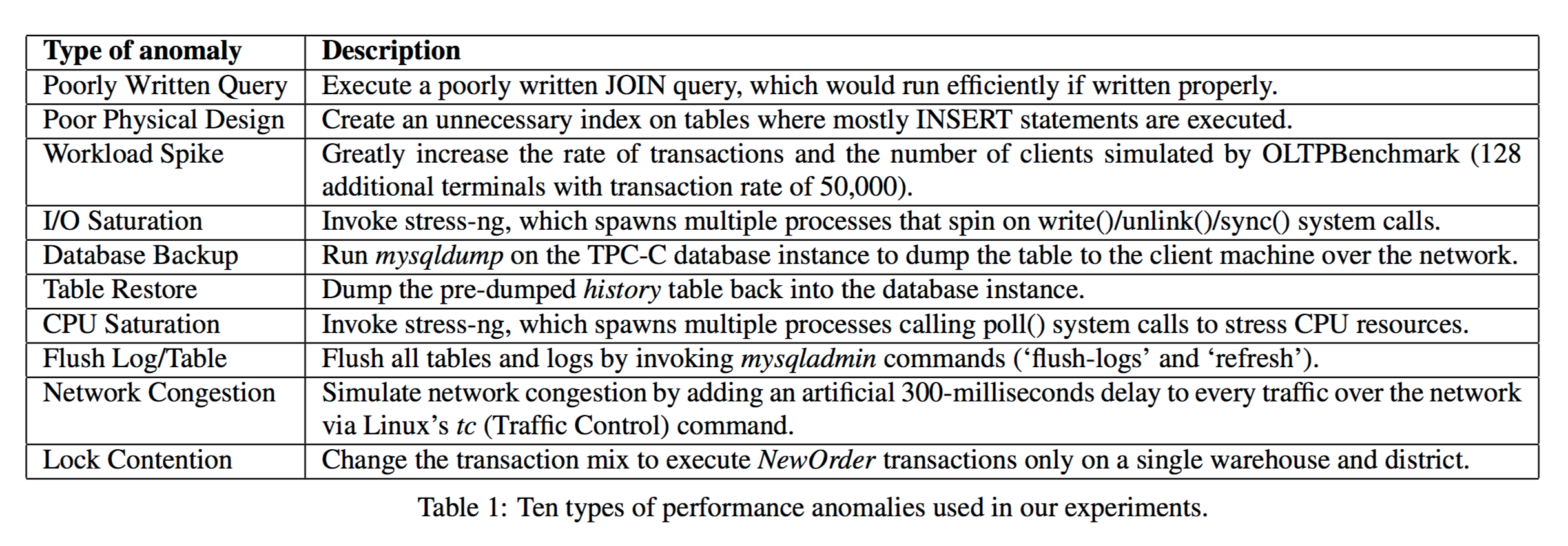
(click to enlarge)
For details, I refer you to the full paper. The short version is:
Our extensive experiments show that our algorithm is highly effective in identifying the correct explanations and is more accurate than the state-of-the art algorithm. As a much needed tool for coping with the increasing complexity of today’s DBMS, DBSherlock is released as an open-source module in our workload management toolkit.
Note that the principles used to build DBSherlock are not tied to the domain of database performance explanation in any deep way, so it should be entirely possible to take these ideas and apply them in other contexts – for example: “why has the latency just shot up on requests to this microservice?”

5 thoughts on “DBSherlock: A performance diagnostic tool for transactional databases”
Comments are closed.