Sharing-aware outlier analytics over high-volume data streams Cao et al. SIGMOD 2016

With yesterday’s preliminaries on skyline queries out of the way, it’s time to turn our attention to the Sharing-aware Outlier Processing (SOP) algorithm of Cao et al. The challenge that SOP addresses is that of building a stream-based outlier detection system that can handle large numbers of outlier detection queries simultaneously. It’s easy to image multiple analysts querying the same core data streams, and even a single analyst wanting to run multiple ongoing queries, perhaps with varying parameters.

Thus, a stream processing system must be able to accommodate a large outlier analytics workload composed of hundreds or more requests covering many, if not all, major parameter settings of an outlier query, and thus striving to capture the most valuable outliers in the stream.

We’re talking about a very particular kind of outlier detection here: detecting outlying points (not patterns), and doing so based on a distance measure. It’s easy to detect outliers based on fixed thresholds, but where do you set the threshold? Fixed thresholds are also very sensitive to concept drift.
For distance-based outlier methods,

… an outlier is an object O with fewer than k neighbours in the dataset D, where a neighbor is defined to be any other object in D that is within a distance range r from object O.

In a streaming context we also need to apply sliding window semantics to ensure that outliers are continuously detected based on the most recent portion of the input stream only. This gives us two additional parameter: the window-size w and the slide-size s (time or count based).

Consider for example monitoring for credit fraud in a banking scenario, where we have a stream of transaction data for individuals with similar income levels. The distance parameter r tells us how dissimilar to other transactions the transaction value must be, the k parameter tells us how far from the majority the transaction must be, and the window size tells us over how many days. “Tell me all transactions that have less than 5 peer transactions within £10,000 over the last 7 days.”

When processing many such queries simultaneously a given point may of course be an inlier from the perspective of some queries, and an outlier for others. SOP handles this situation while still preserving the property that each point is processed only once.

As (the) foundation of our solution, we make the important observation that a workload composed of multiple outlier requests with arbitrary parameter settings can be correctly answered by utilizing one single skyband query – a generalization of the well-known skyline concept. Better yet we prove that given one data point, the skyband points discovered by the skyband query are the minimal yet sufficient evidence required to prove its outlier status with respect to all outlier queries in the workload.

Compared to the previous state-of-the-art (running multiple LEAP queries, or the MCOD algorithm) SOP uses three orders of magnitude less CPU and significantly less memory across a wide range of scenarios. “Furthermore, it is the only known method that scales to huge workloads composed of thousands of outlier requests.”

Let’s take a look at how it works…

Turning distance-based outlier detection into a skyband query

Building up to the full solution, we start out with a group of queries that all use the same window size, slide size, and k, but differ in their distance value, r. Recall that a K-Skyband query reports all points that are dominated by no more than K points. To map the anomaly detection queries into a K-Skyband problem, we therefore have to come up with a suitable definition of the domination relationship between any two points in the current data window.

The key observation here is that given any two points p_i and p_j, two key factors, namely their relative arrival time and the distance to the point p under evaluation, determine whether p_i is more important than p_j in terms of evaluating the outlier status of p.

Take all of the queries and arrange them in order of increasing r value, such that r_m represents the distance parameter for the m^th query.

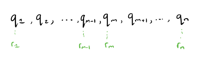
Now consider two points p_i and p, where the distance between them dist(p_i,p) falls between r_m–1 and r_m. You can see the possible queries for which p_i can be a neighbour of p highlighted in blue below (_q_m … q_n).

Above we can also see the possible queries for which p_j can be a neighbour of p, when dist(p_j,p) falls between r_m and r_m+1. From this it is clear that p_i dominates p_j (is more important than p_j) when evaluating queries.

Based on this idea, the normalized distance between two data points p and p_i is defined as m+1, where dist(p,p_i) falls between r_m and r_m+1, with r₀ defined as -∞, and r_n+1 defined as ∞. Henceforth, whenever we refer to distance or ‘dist’ we will mean this normalized distance.

In the time dimension, the younger a data point p_i is, the longer its relationships with p (if any) will persist into the future. Putting the time and distance criteria together, gives us the rules for the domination relationship we are after: point p_i dominates point p_j with respect to point p if

1. p_i.time > p_j.time
2. dist<p,p_i) &leq; dist(p,p_j)
3. dist(p,p_i < n

In other words, given a data point p_i, p_i dominates another point p_j only if p_i expires later than p_j in the current window, and it is not further away from p than p_j. The third condition in the domination rule filters out any data point p_i that is not a neighbour of p for any query in the query set.

Using this definition of domination, a K-skyband query with K specified as k–1 is both sufficient and necessary to continuously determine the outlier sttatus of p with respect to all queries in the set. The skyband query results will always return the k nearest neighbours of p as part of the skyband points. The outlier status of p with respect to each query can then be determined by examining the distance between p and its k-th nearest neighbour. If this falls between r_m and r_m+1 then p is guaranteed to be an outlier for queries {q₁, …, q_m} and an inlier for queries {q_m+1,…, q_n}.

Optimising the skyband query with K-SKY

We could use a traditional K-skyband algorithm for this, such as BBS, but the authors introduce a new K-SKY algorithm that more efficiently supports multiple outlier detection queries. Assuming data points are sorted by arrival time on arrival, then K-SKY only needs to consider distance as later arrivals will never be dominated by earlier arrivals.

K-SKY always conducts the search (for a window) with a ‘later arriving data points first’ order. By this if one data point is not dominated by more than k points in the distance attribute, and thus considered to be a skyband point, then it is not necessary to evaluate it again.

When a window slides, assuming that the slide size is less than the window size (so that windows overlap) we can further reduce computation:

In the sliding window context, the K-SKY search is applied in two situations. First, any new point p that just arrived in the current window needs K-SKY to figure out its skyband points in the current window. Second, an existing point p needs K-SKY to update its skyband points when the stream slides to the current window. In the first situation, for a newly arriving point p, K-SKY has to be conducted from stratch to search for the needed information for p. Instead in the second situation the key observation here is that given the skyband points of the previous window, to acquire the skyband points of the new window only a small fraction of data points in the new window need to be evaluated, namely the new arrivals and the unexpired skyband points of the previous window.

The skyband is computed every time the window moves. Key to the effectiveness of K-SKY is the cost of evaluating each point to determine whether or not it is a skyband point. “Since the number of points examined by K-SKY has already been proven to be minimal, the reduction of the second cost per point is now critical for high performance.” The LSky layered data structure plays a key role in helping to make this determination efficient.

In LSky, skyband points are organized into a layered two dimensional structure that preserves the order among the skyband points in both the distance and the time dimensions. As shown in Fig. 2, the points in each layer have the same distance to point p based on the normalized distance function. The points in the upper layer always have a smaller distance to p than the points in lower layers. Furthermore, in each layer the points are ordered based on their arrival time with the earliest arrival being at the head. By this, skyband points can be quickly expired when the window slides forward in time.

A point p_i to be inserted into the LSky structure is guaranteed to be dominated by points falling in the same layer (since they have been inserted before p_i, and we process the window in reverse time order, they must be more recent) and by points in the layers above it. If in total there are fewer than k such points, then p_i will be a skyband point.

Varying k

So far we’ve assumed all of our queries have the same k. To relax this construct, find the largest k in the query set, and run a skyband query using K-SKY with this k. During LSky processing, it is possible to determine whether a point is an inlier for a given query without introducing any extra overhead. At the end of processing, p is reported as an outlier for all queries that do not mark it as an inlier.

Varying window size

If window sizes vary across queries, but the slide size is constant then all queries will slide to a new window at the same time. We use a similar trick to dealing with varying k, and detect outliers with a single skyband query using the largest window in the query set. Skyband points discovered in this window can be used to answer all queries in the group. An additional outlier status evaluation step is needed for all queries with window size smaller than the maximum. Since I’m running out of space for this write-up, I’ll defer you to section 4.1 in the paper to see how this works. The important thing to note for now is that there is a way to make this extra step efficient.

Varying slide size

A similar trick can be played if window size is held constant, but the slide size varies. Here the single skyband query is issued with the slide size set as the greatest common divisor of the slide sizes of all the anomaly queries.

Putting it all together

SOP first employs a query parser to divide the queries in a query group into sub-groups based on their k parameters. Queries with the same k parameter are grouped into the same sub-group. The queries in each sub-group are then sorted based on their r parameters. The queries with the same r parameters are further sorted based on their window sizes. Then the query parser will create one skyband query for each outlier sub-query group. Its window size is set as the largest window size among the member queries the sub-group. Its slide size is then set as the greatest common divisor of the slide sizes of the member queries. After the query parser transforms the outlier detection queries into skyband queries, the K-SKY algorithm for multiple skyband queries will be applied to detect the skyband points. Then the outlier status evaluator determines the outlier status of each data point with respect to the outlier queries using the inlier rule.

SOP only requires a single pass through new data points, each collecting the minimum evidence needed to prove its outlier status with respect to all queries.

Evaluation

In the most general case, we prepare four workloads composed of 100, 100, 10,000, and 50,000 queries respectively by varying all window-specific and pattern-specific parameters. We observe that similar to the cases of independently varying pattern-specific parameters and window-specific parameters, SOP achieves tremendous gain in CPU utilization compared to (augmented) MCOD and (the non-shared) LELP. Furthermore, SOP shows excellent scalability in the cardinality of the workload.

The memory usage of SOP also consistently outperforms the competition: