Range thresholding on streams Qiao et al. SIGMOD 2016

It’s another streaming paper today, also looking at how to efficiently handle a large volume of concurrent queries over a stream, and also claiming a significant performance breakthrough of several orders of magnitude. We’re looking at a different type of query though, known as a range threshold query. These are queries of the form “tell me when x events have been received with a value within this range.” For example: “Alert me when 100,000 shares of AAPL have been sold in the price range [100,105) starting from now,” and multi-dimensional variants such as “Alert me when 100,000 shares of AAPL have been sold in the price range [100,105), and at the time of sale the NASDAQ index is at 4,600 or lower.”

More formally we’re looking at a data stream of elements e, each with a value v(e) in some d-dimensional space, each dimension with a real-valued domain. Each element also has a weight w(e) – a positive integer which defaults to 1 (counting). A Range Thresholding on Streams (RTS) query q consists of a d-dimensional range specification R_q_ (that a point must fall within to be considered a match), and a threshold τ_q ≥ 1. When sufficient matching elements have been seen such that their combined weight ≥ τ the query matures (and presumably the author of the query is notified). The register operation registers a new query, and terminate stops and eliminates a query.

RTS may look deceptively easy at first glance: whenever a new element e arrives, check whether v(e) is in R_q; if so, increase the weight of R_q by w(e) – clearly a constant time operation overall. This method, unfortunately, stales poorly to the number m of queries running at the same time: now it costs O(m) time to process e. The total cost of processing n stream elements thus becomes a prohibitive quadratic term O(nm). This implies that the method is computationally intractable when m is large. Surprisingly, in spite of the fundamental nature of RTS and the obvious defects of “conventional solutions” like the above, currently no progress has been made to break the quadratic barrier.

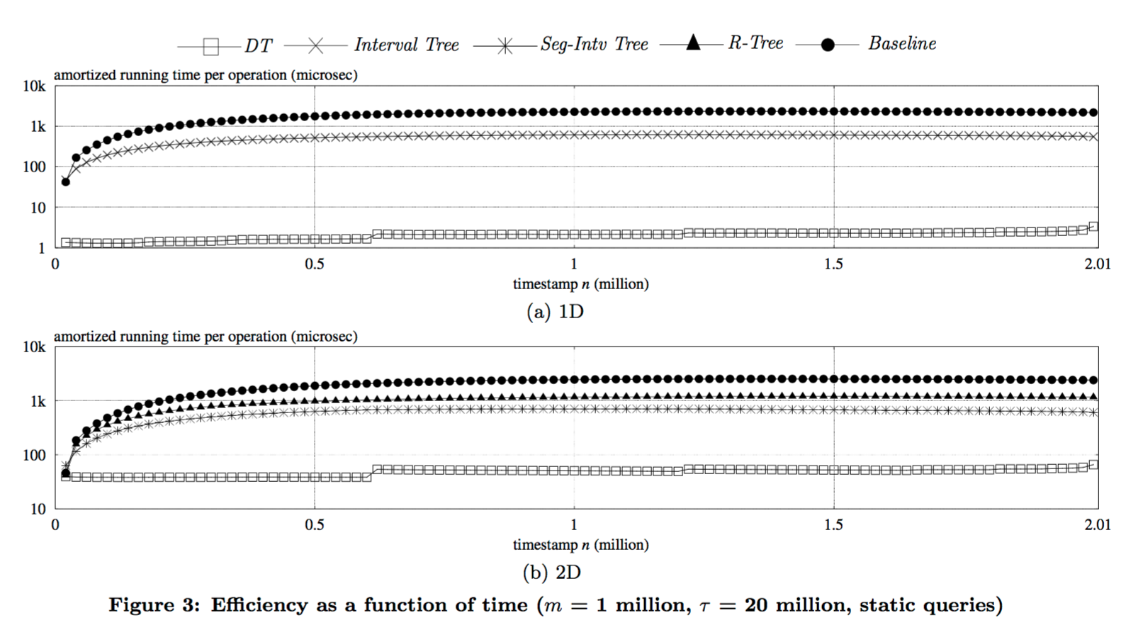
Game on! The authors provide the first algorithm to break the quadratic barrier, giving a solution which is polylogarithmic in O(n+m). That makes this kind of difference when addressing the problem at scale (DT here is Distributed Tracking, the name of the author’s algorithm):

The most crucial discovery is an observation on the connection between RTS and another suprisingly remote problem called distributed tracking. The observation then leads to the development of a novel algorithmic paradigm which, we believe, serves as a powerful weapon for implementing real-time triggers such as RTS.

First therefore, we need to take a brief look at the distributed tracking problem. Then we’ll see how it can be applied to solve the RTS problem when each stream element contains a single value (d=1), and its weight is 1 (i.e. we simply need to count matching events). In addition, we’ll assume initially that all queries are known up-front. We will then add in turn: the ability to register and terminate queries dynamically; matching multi-dimensional elements; and introduced varying weights.

Distributed tracking background

In the distributed tracking problem there are h participants and one coordinator. Communication is only allowed between the coordinator and the participants (participants do not talk directly to each other). Each participant has an integer counter c, and at each time stamp, at most one of the counters is increased by one. The coordinator must report maturity when the sum of all the counter values reaches some threshold τ.

The simple solution is to have each participant send a message to the coordinator whenever its counter increases. This requires O(τ) messages. Whenever τ ≤ 6h we use this solution. For τ > 6h we can do better. First the coordinator calculates a slack value λ, where λ = floor(τ/2h). The coordinator sends the slack value to each participant, and every participant sends a 1-bit signal to the coordinator each time its counter has increased by λ Once the coordinator has received h signals, it collects the precise counter values from all participants and calculates τ‘, τ reduced by the summed count. This completes a round. We keep going until τ’ ≤ 6h, at which point we resort to the simple solution to finish the process.

In the example above where τ is 80 and h = 10, we’ll start off with a slack value of 80/2×10 = 4. When 10 signals have been received the true count must be between 40 and 67 (the other 9 participants could all be one away from sending another signal, 9×3 = 27). The new value of τ will therefore be between 40 and 13, both below 6h, and so the algorithm would then resort to counting individual increments.

This solution is O(h log τ).

A solution to the constrained RTS problem

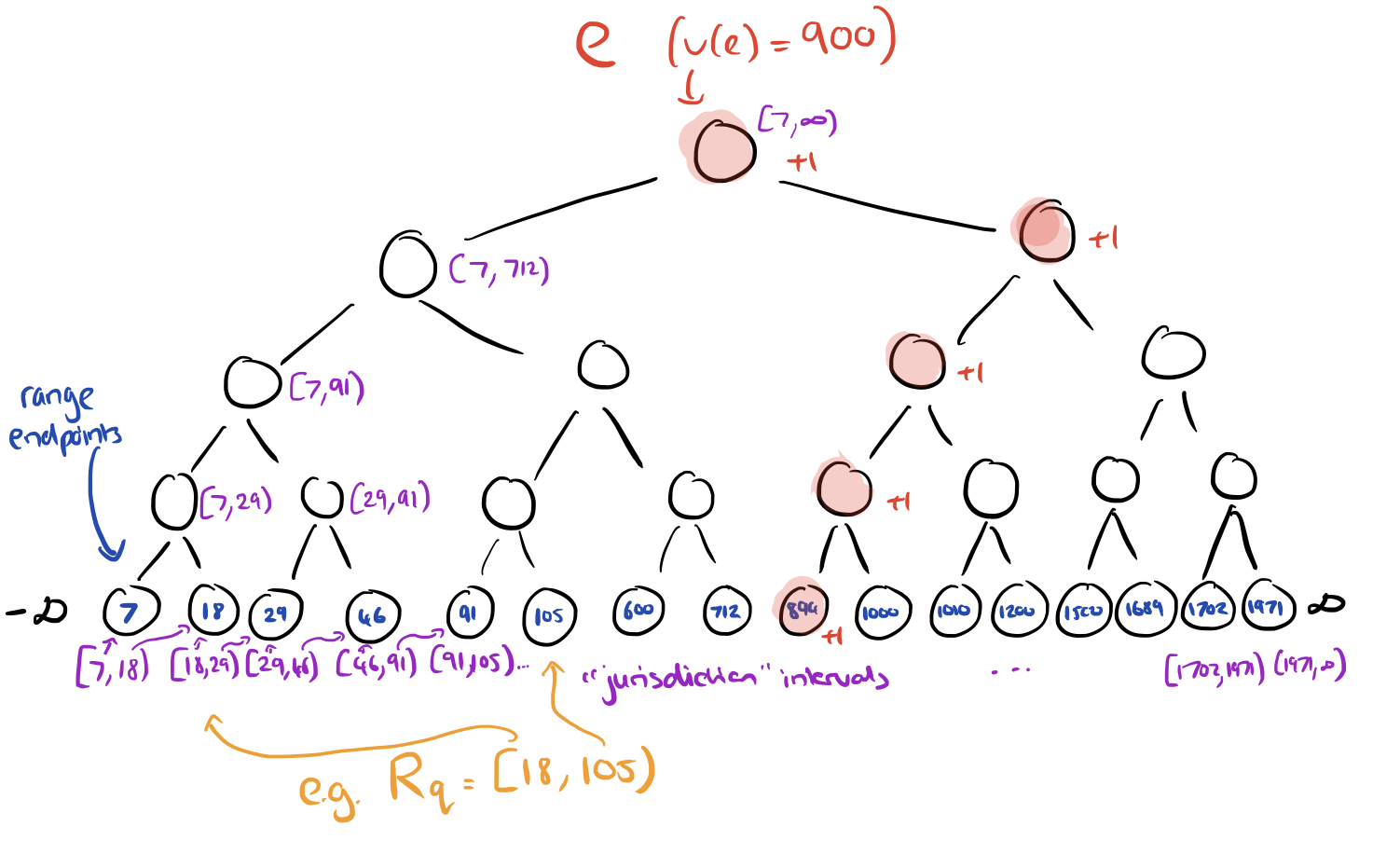
Now we can turn our attention to the RTS problem with a fixed set of queries, d=1, and w=1. Recall that each query has an associated range, e.g. v(e) ∈ [100,105). Create a binary search tree based on the endpoints of those range intervals. This tree will have height O(log m).

Each node in this endpoint tree will have responsibility for a certain portion of the overall range, called its “jurisdiction interval” as shown in the diagram above.

Along comes a stream element e… At each level in the tree, v(e) will fall into the range of exactly one node (unless it is less than the leftmost leaf value, in which case it can be discarded). Each node in the tree maintains a counter, and as e works its way down through the tree, the counter of every node it passes through is incremented. Once e has reached a leaf node it can be discarded (we don’t need to store elements).

The tree itself can be constructed in O(m log m) time, and processing each element takes O(log m) time.

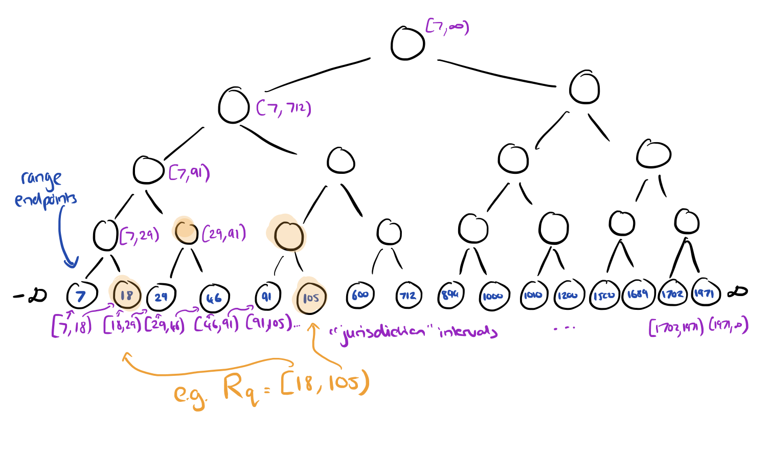
For any given query, define its canonical node set U_q to be the minimum set of nodes with disjoint jurisdiction intervals that cover the range. This will be at most 2 nodes per level of the tree. Continuing our worked example, the canonical node set for a query with range [18,105) is shown below.

Now we can map the RTS problem onto the distributed tracking problem we saw earlier. Let the set of participants h_q be the canonical node set U_q. Let the counters of each node be the counters of the participants, and have the query itself play the role of coordinator. Whenever the counter of a node goes up as an element passes through the tree, treat this as if the counter of the participant has gone up by one.

Every query therefore has its own distributed tracking instance, so conceptually there are m such instances executing concurrently. The maintenance of node counters is common to every instance. When a node counter changes, we should inspect the condition for all queries that include that node in their canonical node set. If we did that though, we’d be back to essentially quadratic time again. Instead for each node we maintain a min_heap per node of all the queries including that node in their canonical set, ordered by the future value of the node counter when the next signal should be sent. Now it suffices only to check against the top entry on the heap, and if the counter has reached that value, send the signal and discard the entry from the heap.

When a query matures, its entry is removed from the heaps of all of its canonical nodes. As more and more queries mature, the space consumed by matured queries needs to be reclaimed at some point. Once the number of currently alive queries has decreased to m/2 (i.e. half of the queries have matured) then a global rebalancing happens and the endpoint query tree is rebuilt using just the currently alive queries (which will have their thresholds adjusted accordingly for the new tree).

See section 4 of the paper for an analysis of the time complexity of this algorithm.

Dynamic queries

Coping with query termination is easy – simply follow the same process as above for when a query matures. When registering a new query, we must insert its endpoints into the tree, which may trigger tree rebalancing operations. This rebalancing can upset the canonical node sets of many queries.

We circumvent this problem by resorting to another, much more practical algorithmic technique called the logarithmic method. It is a generic framework that allows one to convert a semi-dynamic structure supporting only deletions to a fully-dynamic structure that is able to support both deletions and insertions.

In brief, this consists of maintaining g endpoint trees, where g = O(log m). We start out with one tree, and a new tree is created each time the number of alive queries reaches a new power of 2. The first tree has capacity for one query, the second for two queries, the third for 4 queries, and so on. When a new query comes along to be registered, we find the first tree, Τ_j with spare capacity (creating it if needed). Then the queries from all trees up to and including Τ_j are rebuilt into a new Τ_j (and all trees prior to j are reset to empty). The target thresholds for the pre-existing queries are adjusted appropriately when they are placed into the new tree.

Multi-dimensional elements

To deal with multi-dimensional elements (queries along more than one dimension), we can follow the principles set out so far:

• Partition the search region R_q (i.e., an interval when d = 1) into O(1) components, for each of which the number of elements within is kept precisely at a node.
• Many queries can share the same components such that the total number of distinct components is O(m_alive).

When d = 1 we used a binary tree to partition the search region. For d > 1 we can borrow ideas from range trees. If d = 2, then each query will specify a 2-dimensional region [x₁,x₂) x [y₁,y₂), meaning that we’re looking for elements where x₁ ≤ v(e).x < x₂ and y₁ ≤ v(e).y < y₂.

Make a binary search tree using the endpoints in the first dimension (x) as before. Now for each node u in this tree, find all the queries that have u in their (x-) canonical node set. Associate u with a second binary tree built on the y-dimension query endpoints from those queries.

Here’s an example:

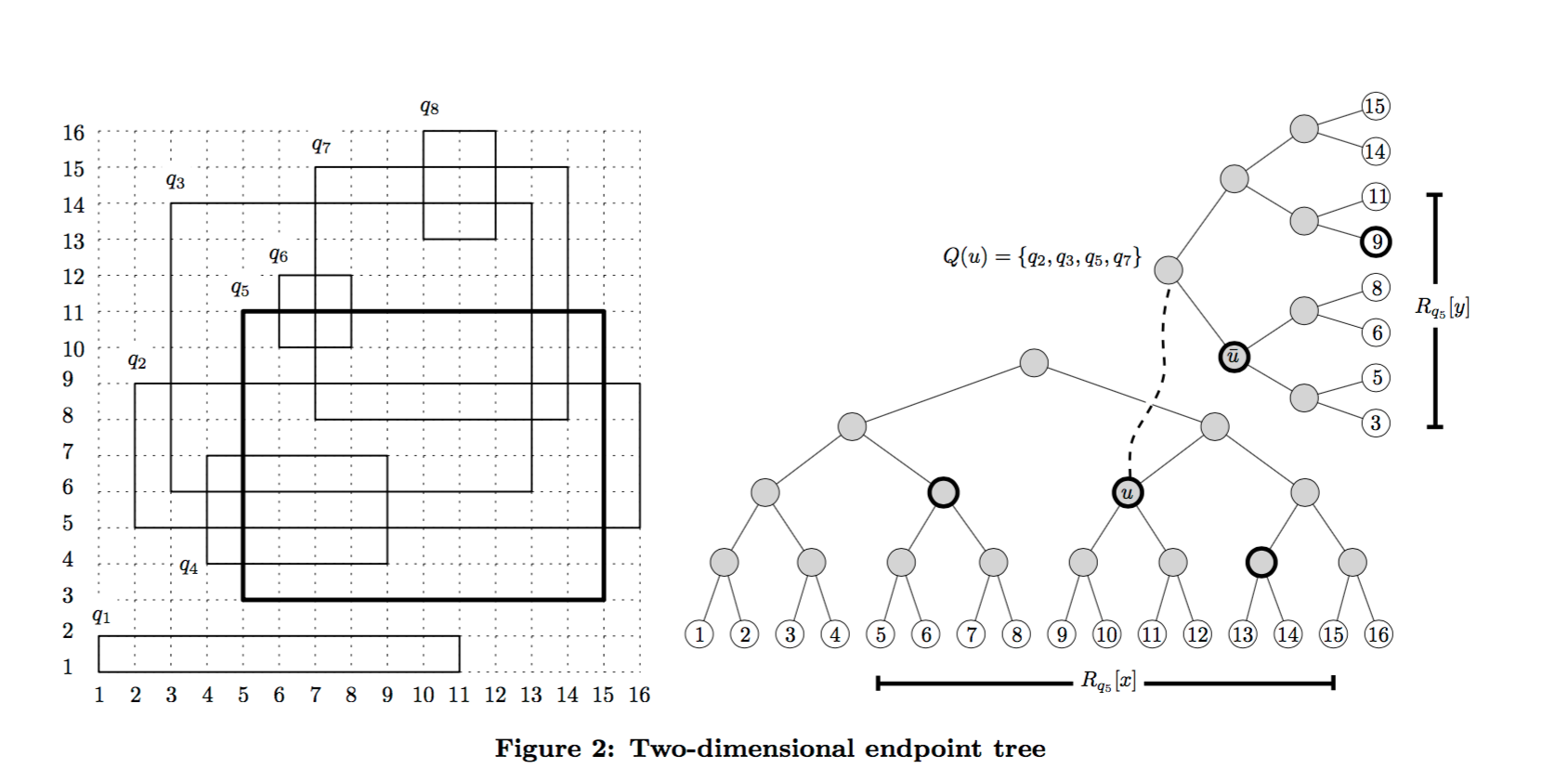
The counters are kept in the secondary trees, and everything else in the algorithm follows the steps previously outlined. If you have more than 2 dimensions, just keep on adding an additional dimension-tree for each tree using the same process.

Varying weights

This relates to a variant of the distributed tracking problem we started with, but where in each time step the (at most one) counter that gets increased, is increased by any positive integer w. A simple approach is to transform this into the unweighted problem by increasing the associated counter by one, w times. The drawback is that we incur O(1) cost every time we increment the counter.

We can revise the distributed tracking problem as follows to address this:

• For τ > 6h, Compute slack in the same way (λ = floor(τ/2h), and send to each participant at the start of the round.
• Send a signal from a participant when its counter has increased by λ since the last signal (as per the previous algorithm), unless the coordinator has announced the end of this round.
• The coordinator collects all counter values when it has received h signals, and also announces that the round is finished.

To reach the final version of the DT-RTS algorithm, replace the orginal distributed tracking algorithm we started with, with this updated version.

The last word

In this paper, we have developed the first algorithm whose running time successfuly escapes the quadratic trap – even better, the algorithm promises computation cost that is near-linear to the input size, up to a polylogarithmic factor. Extensive experimentation has confirmed that the new algorithm, besides having rigourous theoretical guarantees, has excellent performance in practical scenarios, outperforming alternative methods by a factor up to orders of magnitude. It can therefore be immediately leveraged as a reliable fundamental tool for building sophisticated triggering mechanisms in real systems.