Searching and mining trillions of time series subsequences under dynamic time warping – Rakthanmanon et al. SIGKDD 2012
What an astonishing paper this is! By 2012, Dynamic Time Warping had been shown to be the time series similarity measure that generally performs the best for matching, but because of its computational complexity researchers and practitioners often turned to other similarity measures or approximations. For example,
The proliferation of inexpensive low-powered sensors has produced an explosion of interest in monitoring real-time streams of medical telemetry and/or Body Area Network (BAN) data. There are dozens of research efforts in this domain that explicitly state that while monitoring under DTW is desirable, it is impossible. Thus, approximations of, or alternatives to DTW are used. Dozens of suggested workarounds have been suggested…
There is no shortage of work on such measures – table 1 in the 2012 ACM Computing Surveys paper on Time-Series Data Mining lists 27 of them, arranged in four different categories. However, the authors assert:
… after an exhaustive literature search of more than 800 papers, we are not aware of any distance measure that has been shown to outperform DTW by a statistically significant amount on reproducible experiments. Thus DTW is the measure to optimize (recall that DTW subsumes Euclidean distance as a special case).
After all this time (DTW itself is about 40 years old), and all that research effort into alternatives and faster approximations, Rakthanamanon et al. present a collection of four optimisations (collectively called the UCR suite) to DTW that enable exact searching much more quickly than even the current state-of-the-art Euclidean distance search algorithms. As an example,
An influential paper on gesture recognition on multi-touch screens laments that “DTW took 128.6 minutes to run the 14,400 tests for a give subject’s 160 gestures.” However, we can reproduce the results in under 3 seconds.
The UCR suite makes even real-time usage of DTW on low-power devices feasible.
To see this, we created a dataset of one year of electrocardiograms (ECGs) sampled at 256Hz. We created this data by concatenating the ECGs of more than two hundred people, and thus we have a highly diverse dataset, with 8,518,554,188 data points. We created a query by asking USC cardiologist Dr. Helga Van Herle to produce a query she searches for on a regular basis, she created an idealized Premature Ventricular Contraction (PVC)….
The UCR-DTW based search completed in 18 minutes, whereas the state-of-the-art DTW solution required 49.2 hours! On a standard desktop machine, the results were computed 29,919x faster than real-time (256Hz), suggesting that real-time DTW is indeed tenable on low-power devices.
I said in the introduction that this is an astonishing paper. And it is truly impressive that after so much prior time and research had been expended on the problem, the authors were able to make improvements of such magnitude. But what makes it astonishing, is that when you see the four optimisations, they are all actually very straightforward (with the benefit of hindsight ;) ). These results are not the product of super-sophisticated algorithms, but rather the application of solid engineering thinking backed up by careful evaluations. And all credit to the authors for it.
For the rest of this write-up, first let’s take a look at DTW itself and the known optimisations prior to the publication of this paper, and then we can dive into the four optimisations in the UCR suite.
A dynamic time warping primer
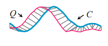
Lets start by considering the Euclidean Distance (ED) between some query Q (find me parts of the time series that look like this), and a candidate subsequence C of the time series we want to match against. This is very straightforward to calculate – we just sum the squares of the distances between the Q and C at each time point and take the square root.

In this example you can see that Q and C have similar but slightly out of phase peaks. We could get a better similarity measure of Q and C if instead of comparing Q and C directly at the same points (the vertical grey lines above), we constructed a mapping between Q and C that better aligns the two series first. This is what DTW does. Such a mapping is called a warping path. The Euclidean Distance therefore, can be viewed simply as a special case of DTW.
To align two sequences using DTW, an n-by-n matrix is constructed, with the (ith,jth) element of the matrix being the Euclidean Distance d(qi,cj) between the points qi and cj. A warping path P is a contiguous set of matrix elements that defines a mapping between Q and C.

The warping path that defines the alignment between the two time series is subject to several constraints. For example, the warping path must start and finish in diagonally opposite corner cells of the matrix, the steps in the warping path are restricted to adjacent cells, and the points in the warping path must be monotonically spaced in time. In addition, virtually all practitioners using DTW also constrain the warping path in a global sense by limiting how far it may stray from the diagonal. A typical constraint is the Sakoe-Chiba Band which states that the warping path cannot deviate more than R cells from the diagonal.
Four optimisations to the basic DTW sequential search are as follows:
- Eliminate the square roots. Both DTW and ED have a square root calculation, but you can omit it without changing the relative rankings of nearest neighbours. When the user submits a range query, the implementation simply squares the desired value, performs the search, and then takes the square root of distances found before presenting the answers.
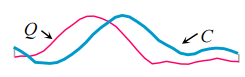
- Prune using cheap to compute lower bounds. Consider the query and candidate below. We can quickly look ( O(1) ) at the first and last data points in the sequence and see that a lower bound on DTW can be quickly determined from their Euclidean distances. This is known as the LB_KimFL lower bound.
The related LB_Keogh lower bound can be computed in O(n) and uses the Euclidean distance between the candidate sequence C and the closer of {U,L} as the lower bound.

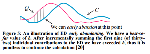
- Abandon ED and LB_Keogh computation early. “During the computation of the Euclidean distance or the LB_Keogh lower bound, if we note that the current sum of the squared differences between each pair of corresponding data points exceeds the best-so-far we can stop the calculation since the exact distance must also exceed it.”
- Abandon DTW early.
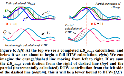
If we have computed a full LB_Keogh lower bound, but we find that we must calculate the full DTW, there is still one trick left up our sleeves. We can incrementally compute the DTW from left to right, and as we incrementally calculate from 1 to K, we can sum the partial DTW accumulation with the LB_Keogh contribution from K+1 to n.
The sum of the partial DTW with the remaining LB_Keogh bound is a lower bound to the true DTW distance, and again we can stop early if this exceeds the best-so-far. “Moreover, with careful implementation the overhead costs are negligible.”
The UCR suite of optimisations
Now that we’ve covered the base DTW algorithm, and the four prior known optimisations, let’s look at the four additional optimisations introduced by the authors in their UCR suite.
Abandon normalisation early
Something I’ve omitted to mention so far, is that you need to normalize both Q and each candidate subsequence C before computing the DTW similarity. It is not sufficient to normalize the entire dataset. “While this may seem intuitive, and was explicitly emprically demonstrated a decade ago in a widely cited paper, many research efforts do not seem to realize this.”
To the best of our knowledge, no one has ever considered optimizing the normalization step. This is suprising, since it takes slightly longer that computing the Euclidean distance itself. Our insight here is that we can interleave the early abandoning calculations of Euclidean distance (or LB_Keogh) with the online Z-normalization… Thus if we can early abandon, we are pruning not just distance calculation, but also normalization steps.
For a window of size m, all you need to do is keep two running sums of the long time series that have a lag of exactly m values. From this you can easily compute the mean and standard deviation:
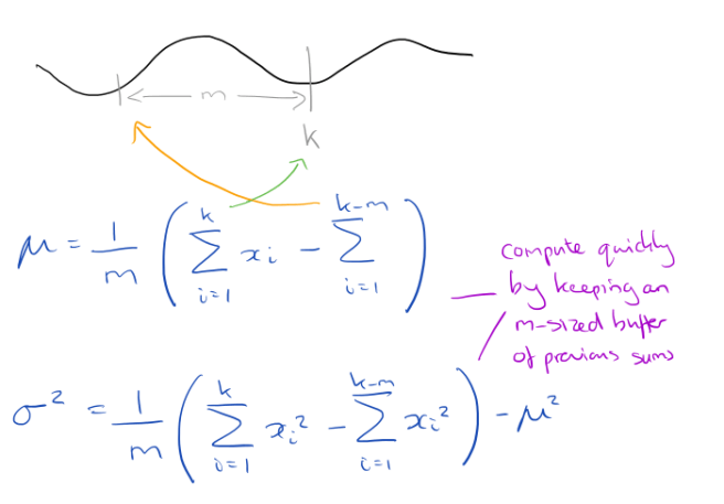
To avoid problems with accumulated floating-point error, once in every one million subsequences a complete Z-normalization is forced to “flush out” any accumulated error.
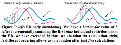
Reorder early abandoning
It was previous assumed that early abandoning should proceed left-to-right. But maybe there is a better ordering? Intuitively, we’d like to incrementally sum the biggest differences first, which would let us abandon even earlier (i.e. with fewer calculations). For example, in left-to-right order in the left illustration below, we can abandon after nine steps, but in the right illustration we can abandon after only five steps.
But how do we know which points will have the biggest differences?
We conjecture that the universal optimal ordering is to sort the indices based on the absolute values of the Z-normalized Q. The intuition behind this idea is that the value at Qi will be compared to many Ci‘s during a search. However, for subsequence search, with Z-normalized candidates, the distribution of many Ci‘s will be Gaussian, with a mean of zero. Thus, the sections of the query that are the furthest from the mean, zero, will on average have the largest contributions to the distance measure.
This intuition was tested by comparing a query heartbeat to one million other randomly chosen ECG sequences, and comparing what the best ordering would have been, with the one predicted by the conjecture. “We found the rank correlation is 0.999.”
Use cascading lower bounds
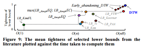
There are several different ways of calculating lower bounds. Each of these has a certain pruning power, and a certain cost to compute (e.g. we saw LB_Kim and LB_Keogh earlier). At least 18 different lower bound mechanisms have been proposed, and the authors implemented all of them and tested against fifty different datasets.
Following the literature, we measured the tightness of each lower bound as LB(A,B) / DTW(A,B) over 100,000 randomly sampled subsequences A and B of length 256. The reader will appreciate that a necessary condition for a lower bound to be useful is for it to appear on the “skyline” shown with a dashed line; otherwise there exists a faster-to-compute bound that is at least as tight, and we should use that instead.
Which lower bound from the skyline should be used though?
Our insight is that we should use all of them in a cascade. We first use the O(1) LB_Kim_FB, which while a very weak lower bound prunes many objects. If a candidate is not pruned at this stage, we compute the LB_KeoghEQ. Note that as discussed in sections… we can incrementally compute this: thus, we may be able to abandon anywhere between O(1) and O(n) time. If we complete this lower bound without exceeding the best-so-far, we compute LB_KeoghEC. If this bound does not allow us to prune, we then start the early abandoning calculation of DTW.
Reversing the roles of query and candidate when computing lower bounds
In standard practice LB_Keogh builds the envelope around the query. This only needs to be done once, saving the time and space otherwise needed to build the envelope around each candidate. But with the skyline pruning just described, we can selectively calculate LK_KeoghEC in a ‘just-in-time’ fashion only if all other lower bounds fail to prune. This enables an optimisation whereby the envelope is built around the candidate (that has survived pruning).
This removes space overhead, and as we will see, the time overhead pays for itself by pruning more full DTW calculations. Note that in general, LB_KeoghEQ ≠ LB_KeoghEC and that on average each one is larger about half the time.
Results
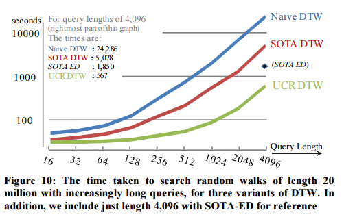
Querying against a random-walk dataset, the UCR optimisations with Euclidean distance or full DTW significantly outperform the state-of-the-art (SOTA):

The longer the query, the better the relative improvement:
The result of long queries with EEG data, and very long queries with DNA data are equally impressive.
With oversampled data (e.g. ECGs sampled at 256Hz, vs current machines sampling at 2,048Hz) the search can be speed up even more by provisionally searching in a downsampled version of the data to provide a quick best-so-far, that can then be projected back into the original space to prime a low best-so-far value to be used in early abandoning.
We have shown our suite of ideas is 2 to 164 times faster than the true state of the art, depending on the query/data. However, based on the quotes from papers we have sprinkled throughout this work, we are sometimes more than 100,000 times faster than recent papers…. much of the recent pessimism about using DTW for real-time problems was simply unwarranted.

Seems to be faster than dtw:
http://www2.informatik.hu-berlin.de/~schaefpa/bossVS/
Hth
Regards
Bernd
I’m clearly going to have to do another week of time series papers soon! I want to cover SAX, and some of the deep learning approaches to classification, and this looks to be another really interesting paper – thanks for the pointer!
What do you mean “Seems to be faster than dtw….”.
There is no need for ‘seems’, you can just do experiments.
(which, by the way, we have, lots of them). If you read the paper you will see that DTW can be computed within a factor of two of Gods algorithm.
I
—-
Many thanks to Adrian, for his very kinds words. I am very proud of this paper, we had an amazing team working on this.