Dynamic word embeddings for evolving semantic discovery Yao et al., WSDM’18
One of the most popular posts on this blog is my introduction to word embeddings with word2vec (‘The amazing power of word vectors’). In today’s paper choice Yao et al. introduce a lovely extension that enables you to track how the meaning of words changes over time. It would be a superb tool for analysing brands for example.
Human language is an evolving construct, with word semantic associations changing over time. For example,
applewhich was traditionally only associated with fruits, is now also associated with a technology company. Similarly the association of names of famous personalities (e.g.,trump) changes with a change in their roles. For this reason, understanding and tracking word evolution is useful for time-aware knowledge extraction tasks….
Let’s go straight to some examples of what we’re talking about here:
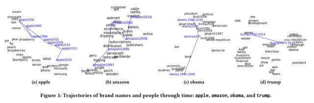
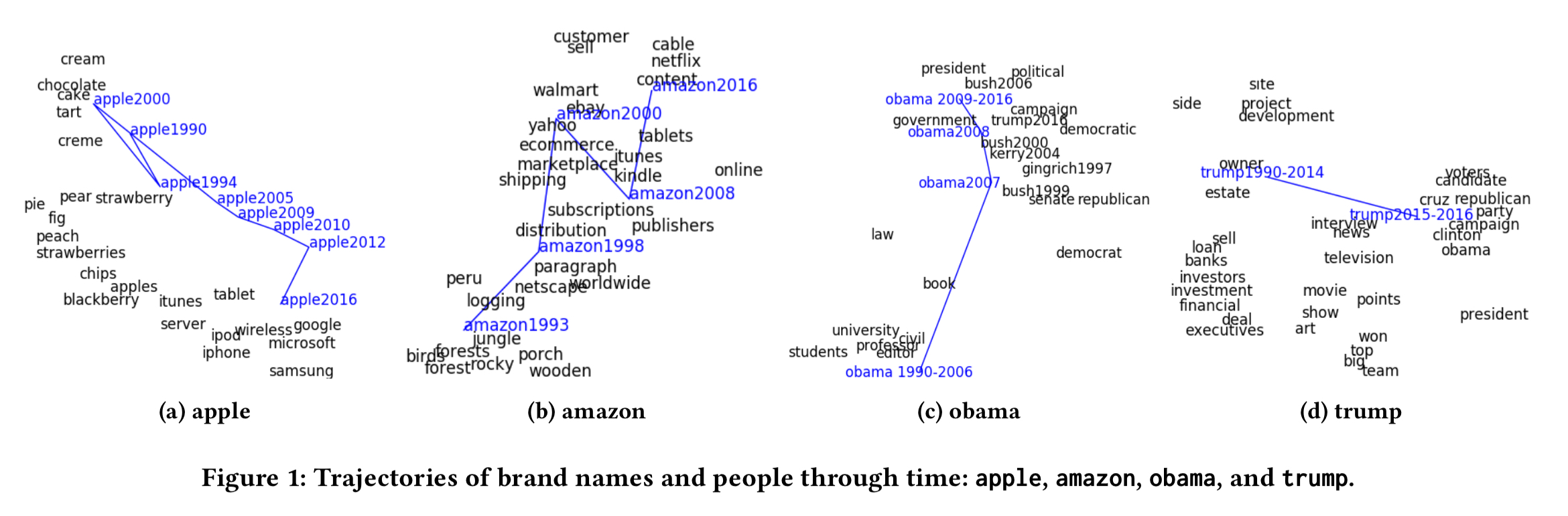
(Enlarge)
Consider the trajectory of ‘apple’: in 1994 it’s most closely associated with fruits, and by 2000 changing dietary associations can be seen, and apple is associated with the less healthy ‘cake,’ ‘tart,’ and ‘cream.’ From 2005 through 2016 though, the word is strongly associated with Apple the company, and moreover you can see the changing associations with Apple over time, from ‘iTunes’ to Google, Microsoft, Samsung et al..
Likewise ‘amazon’ moves from a river to the company Amazon, and ‘Obama’ moves from his pre-presidential roles to president, as does ‘Trump.’
These embeddings are learned from articles in The New York Times between 1990 and 2016. The results are really interesting (we’ll see more fun things you can do with them shortly), but you might be wondering why this is hard to do. Why not simply divide up the articles in the corpus (e.g., by year), learn word embeddings for each partition (which we know how to do), and then compare them?
What makes this complicated is that when you learn an embedding for a word in one time window (e.g., ‘bank’), there’s no guarantee that the embedding will match that in another time window, even if there is no semantic change in the meaning of the word across the two. So the meaning of ‘bank’ in 1990 and 1995 could be substantially the same, and yet the learned embeddings might not be. This is known as the alignment problem.
A key practical issue of learning different word embeddings for different time periods is alignment. Specifically, most cost functions for training are invariant to rotations, as a byproduct, the learned embeddings across time may not be placed in the same latent space.
Prior approaches to solving this problem first use independent learning as per our straw man, and then post process the embeddings in an alignment phase to try and match them up. But Yao et al. have found a way to learn temporal embeddings in all time slices concurrently, doing away with the need for a separate alignment phase. The experimental results suggests that this yields better outcomes that the prior two-step methods, and the approach is also robust against data sparsity (it will tolerate time slices where some words are rarely present or even missing).
Temporal word embeddings
Recall that underpinning word embeddings is the idea of a co-occurrence matrix (see ‘GloVe: Global vectors for word representation’) capturing the pointwise mutual information (PMI) between any two words in the vocabulary. Given a corpus 

Where 


The learned embedding vectors for w and c, 


Adding a temporal dimension to this, for each time slice t the positive PMI matrix 

And the temporal word embeddings 

This still doesn’t solve the alignment problem though. To encourage alignment, the authors cast finding temporal word embeddings as the solution to the following joint optimisation problem:
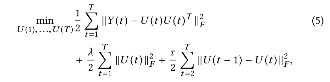
where 

- The penalty term
enforces low-rank data fidelity as has been widely adopted in previous work
- The smoothing term
encourages the word embeddings to align. The parameter
controls how fast the embeddings can change over time.
This is decomposed to solve the objective function across time for each
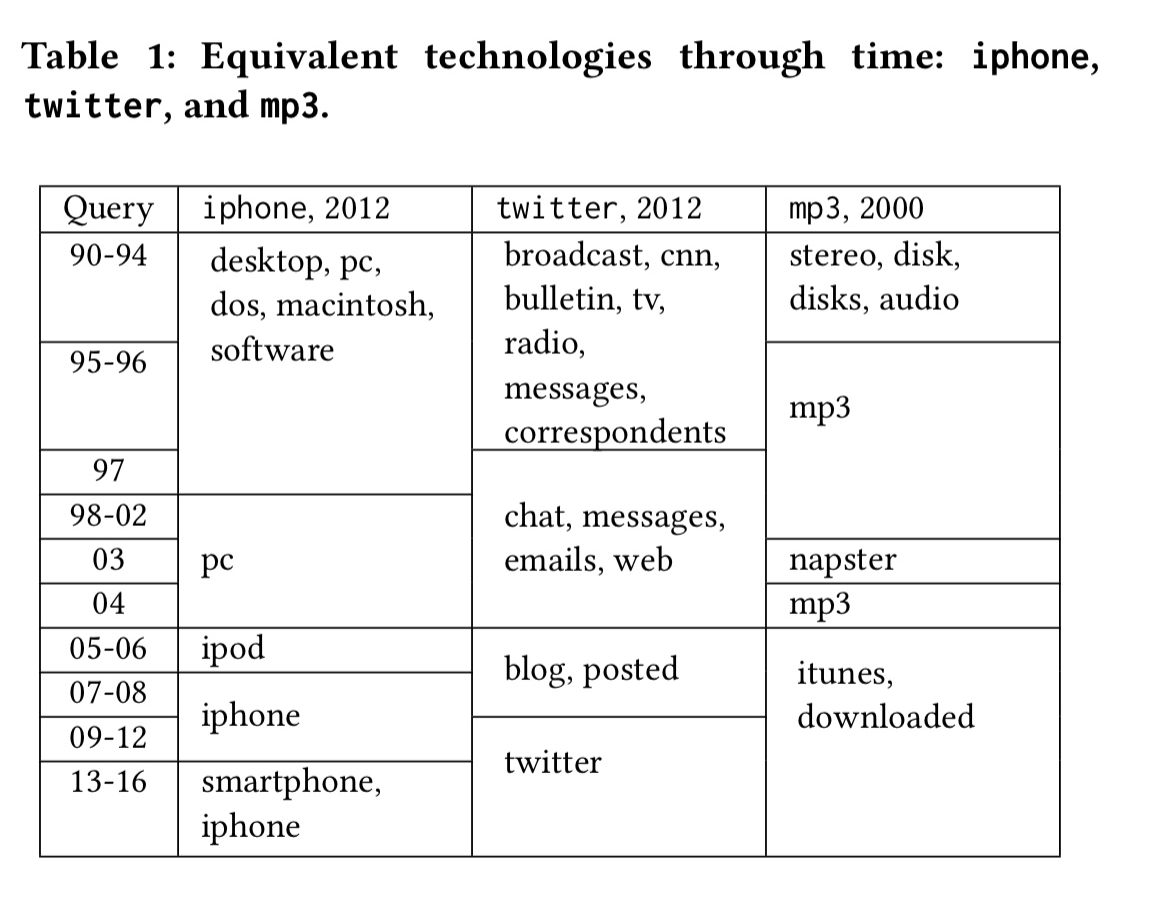
Finding equivalent terms over time
Let’s return to the fun things you can do with the resulting embeddings. Here’s an example of finding conceptually equivalent items or people over time. For example, the closest equivalent to the ’iPhone’ as of 2012 was ‘pc’ in 2003, and by 2013-16 it was ‘smartphone.’ Likewise back in 1990-94 the equivalents of twitter were ‘broadcast’, ‘cnn’, ‘radio’ etc.. In the ‘mp3’ column you can clearly see associations with the dominant form of music consumption in the given time periods.
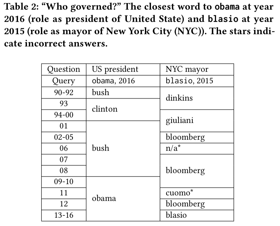
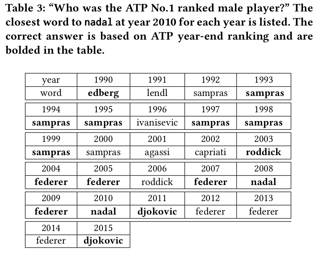
We can do a similar thing asking who played a certain political role in a given year:
Even more impressive, is this search for equivalence in sport by looking for the ATP No. 1 ranked male tennis player in a given year. Here we’re asking, who played the same role that Nadal did in the year 2010?
Tracking popularity over time
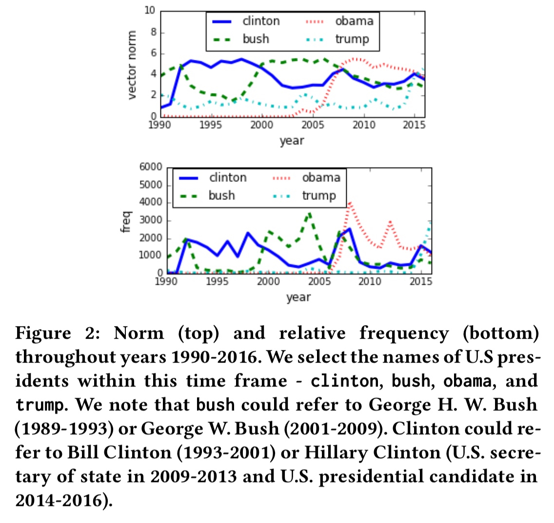
The learned word vector norms across times grow with word frequency, and can be viewed as a time series for detecting trending concepts with more robustness than word frequency.
Generally, comparing to frequencies which are more sporadic and noisy, we note that the norm of our embeddings encourages smoothness and normalization while being indicative of the periods when the corresponding words were making news rounds.
Here’s a comparison of norms (top chart) and word frequency (bottom chart) for the names of US presidents over time.
The last word
Our proposed method simultaneously learns the embeddings and aligns them across time, and has several benefits: higher interpretability for embeddings, better quality with less data, and more reliable alignment for across-time querying.

Adrian, The WordPress typesetting of maths is getting annoying.
Yes, it’s really annoying! I’d consider moving platform if it wasn’t so much effort, still hoping wp.com will fix it… https://twitter.com/adriancolyer/status/966584058275860480
You could try Github Pages with Jenkins, you can serve any type of static website with it. Might be a pain for the comments and I don’t know how they’d handle your traffic, but it’s an option I guess.
Anyway, thanks for your amazing work! Congrats from France :)
Thanks for sharing this! I’m planning to explore this approach with very specific structured data sets and technology terms used within those domains (less ambiguity). However, I’m concerned that the authors are all CS/Engineering and there isn’t a single Linguist or other Social Scientist involved in this research. I’m also concerned that the paper may be misusing the idea of “meaning” with regards to word2vec. When I’ve shared this I’ve rephrased it as “the evolving context of terms used in the NY Times”. Ultimately word2vec only provides insights into what words are used together, but whether that is sufficient for semantic meaning is debatable.
This is great, but I wasn’t sure how you asked questions of the word embeddings. For example, you asked “who played the same role that Nadal did in the year 2010?”. How was that query implemented? Did you use a natural language question answering system?