For today’s post, I’ve drawn material not just from one paper, but from five! The subject matter is ‘word2vec’ – the work of Mikolov et al. at Google on efficient vector representations of words (and what you can do with them). The papers are:

• Efficient Estimation of Word Representations in Vector Space – Mikolov et al. 2013
• Distributed Representations of Words and Phrases and their Compositionality – Mikolov et al. 2013
• Linguistic Regularities in Continuous Space Word Representations – Mikolov et al. 2013
• word2vec Parameter Learning Explained – Rong 2014
• word2vec Explained: Deriving Mikolov et al’s Negative Sampling Word-Embedding Method – Goldberg and Levy 2014

From the first of these papers (‘Efficient estimation…’) we get a description of the Continuous Bag-of-Words and Continuous Skip-gram models for learning word vectors (we’ll talk about what a word vector is in a moment…). From the second paper we get more illustrations of the power of word vectors, some additional information on optimisations for the skip-gram model (hierarchical softmax and negative sampling), and a discussion of applying word vectors to phrases. The third paper (‘Linguistic Regularities…’) describes vector-oriented reasoning based on word vectors and introduces the famous “King – Man + Woman = Queen” example. The last two papers give a more detailed explanation of some of the very concisely expressed ideas in the Milokov papers.

Check out the word2vec implementation on Google Code.

What is a word vector?

At one level, it’s simply a vector of weights. In a simple 1-of-N (or ‘one-hot’) encoding every element in the vector is associated with a word in the vocabulary. The encoding of a given word is simply the vector in which the corresponding element is set to one, and all other elements are zero.

Suppose our vocabulary has only five words: King, Queen, Man, Woman, and Child. We could encode the word ‘Queen’ as:

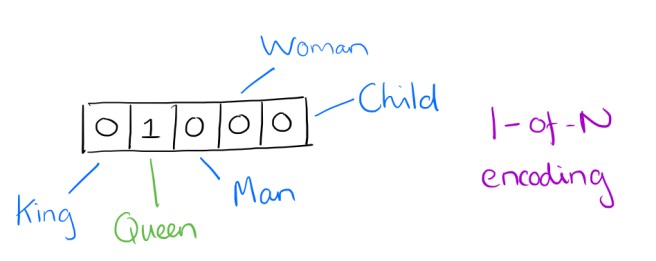
Using such an encoding, there’s no meaningful comparison we can make between word vectors other than equality testing.

In word2vec, a distributed representation of a word is used. Take a vector with several hundred dimensions (say 1000). Each word is representated by a distribution of weights across those elements. So instead of a one-to-one mapping between an element in the vector and a word, the representation of a word is spread across all of the elements in the vector, and each element in the vector contributes to the definition of many words.

If I label the dimensions in a hypothetical word vector (there are no such pre-assigned labels in the algorithm of course), it might look a bit like this:

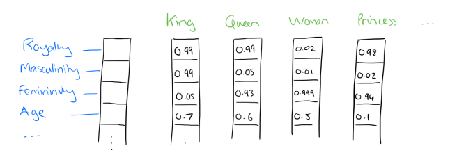
Such a vector comes to represent in some abstract way the ‘meaning’ of a word. And as we’ll see next, simply by examining a large corpus it’s possible to learn word vectors that are able to capture the relationships between words in a surprisingly expressive way. We can also use the vectors as inputs to a neural network.

Reasoning with word vectors

We find that the learned word representations in fact capture meaningful syntactic and semantic regularities in a very simple way. Specifically, the regularities are observed as constant vector offsets between pairs of words sharing a particular relationship. For example, if we denote the vector for word i as x_i, and focus on the singular/plural relation, we observe that x_apple – x_apples ≈ x_car – x_cars, x_family – x_families ≈ x_car – x_cars, and so on. Perhaps more surprisingly, we find that this is also the case for a variety of semantic relations, as measured by the SemEval 2012 task of measuring relation similarity.

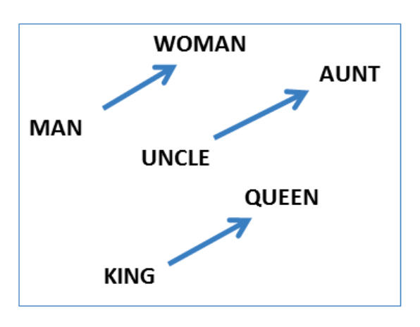
The vectors are very good at answering analogy questions of the form a is to b as c is to ?. For example, man is to woman as uncle is to ? (aunt) using a simple vector offset method based on cosine distance.

For example, here are vector offsets for three word pairs illustrating the gender relation:

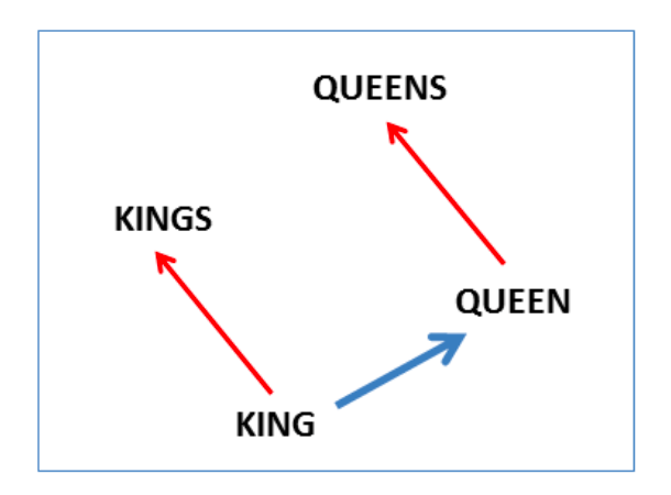
And here we see the singular plural relation:

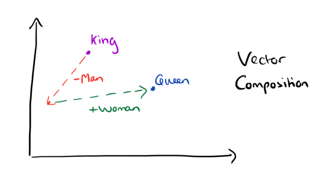
This kind of vector composition also lets us answer “King – Man + Woman = ?” question and arrive at the result “Queen” ! All of which is truly remarkable when you think that all of this knowledge simply comes from looking at lots of word in context (as we’ll see soon) with no other information provided about their semantics.

Somewhat surprisingly, it was found that similarity of word representations goes beyond simple syntatic regularities. Using a word offset technique where simple algebraic operations are performed on the word vectors, it was shown for example that vector(“King”) – vector(“Man”) + vector(“Woman”) results in a vector that is closest to the vector representation of the word Queen.

Vectors for King, Man, Queen, & Woman:

The result of the vector composition King – Man + Woman = ?

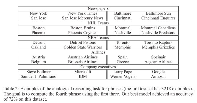
Here are some more results achieved using the same technique:

Here’s what the country-capital city relationship looks like in a 2-dimensional PCA projection:

Here are some more examples of the ‘a is to b as c is to ?’ style questions answered by word vectors:

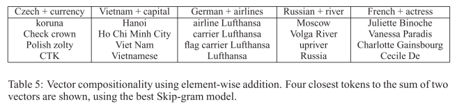
We can also use element-wise addition of vector elements to ask questions such as ‘German + airlines’ and by looking at the closest tokens to the composite vector come up with impressive answers:

Word vectors with such semantic relationships could be used to improve many existing NLP applications, such as machine translation, information retrieval and question answering systems, and may enable other future applications yet to be invented.

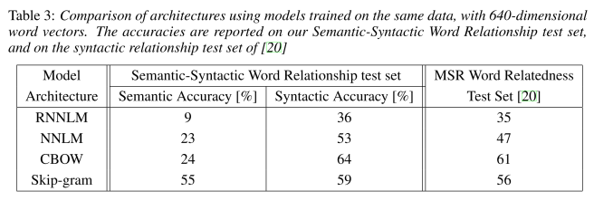
The Semantic-Syntatic word relationship tests for understanding of a wide variety of relationships as shown below. Using 640-dimensional word vectors, a skip-gram trained model achieved 55% semantic accuracy and 59% syntatic accuracy.

Learning word vectors

Mikolov et al. weren’t the first to use continuous vector representations of words, but they did show how to reduce the computational complexity of learning such representations – making it practical to learn high dimensional word vectors on a large amount of data. For example, “We have used a Google News corpus for training the word vectors. This corpus contains about 6B tokens. We have restricted the vocabulary size to the 1 million most frequent words…”

The complexity in neural network language models (feedforward or recurrent) comes from the non-linear hidden layer(s).

While this is what makes neural networks so attractive, we decided to explore simpler models that might not be able to represent the data as precisely as neural networks, but can posssible be trained on much more data efficiently.

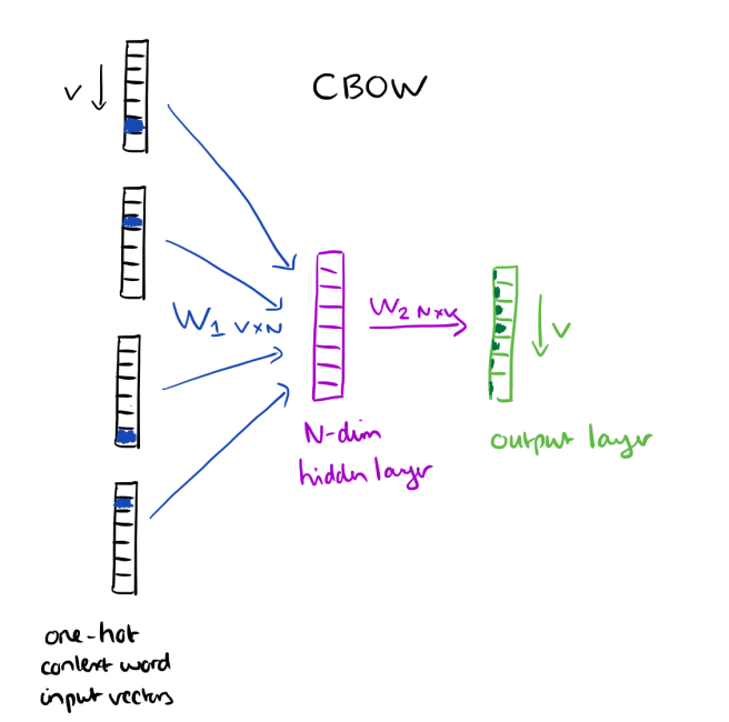
Two new architectures are proposed: a Continuous Bag-of-Words model, and a Continuous Skip-gram model. Let’s look at the continuous bag-of-words (CBOW) model first.

Consider a piece of prose such as “The recently introduced continuous Skip-gram model is an efficient method for learning high-quality distributed vector representations that capture a large number of precises syntatic and semantic word relationships.” Imagine a sliding window over the text, that includes the central word currently in focus, together with the four words and precede it, and the four words that follow it:

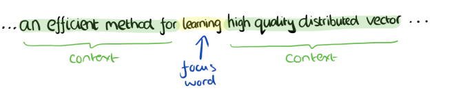
The context words form the input layer. Each word is encoded in one-hot form, so if the vocabulary size is V these will be V-dimensional vectors with just one of the elements set to one, and the rest all zeros. There is a single hidden layer and an output layer.

The training objective is to maximize the conditional probability of observing the actual output word (the focus word) given the input context words, with regard to the weights. In our example, given the input (“an”, “efficient”, “method”, “for”, “high”, “quality”, “distributed”, “vector”) we want to maximize the probability of getting “learning” as the output.

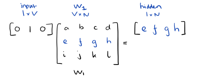
Since our input vectors are one-hot, multiplying an input vector by the weight matrix W₁ amounts to simply selecting a row from W₁.

Given C input word vectors, the activation function for the hidden layer h amounts to simply summing the corresponding ‘hot’ rows in W₁, and dividing by C to take their average.

This implies that the link (activation) function of the hidden layer units is simply linear (i.e., directly passing its weighted sum of inputs to the next layer).

From the hidden layer to the output layer, the second weight matrix W₂ can be used to compute a score for each word in the vocabulary, and softmax can be used to obtain the posterior distribution of words.

The skip-gram model is the opposite of the CBOW model. It is constructed with the focus word as the single input vector, and the target context words are now at the output layer:

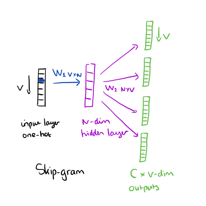
The activation function for the hidden layer simply amounts to copying the corresponding row from the weights matrix W₁ (linear) as we saw before. At the output layer, we now output C multinomial distributions instead of just one. The training objective is to mimimize the summed prediction error across all context words in the output layer. In our example, the input would be “learning”, and we hope to see (“an”, “efficient”, “method”, “for”, “high”, “quality”, “distributed”, “vector”) at the output layer.

Optimisations

Having to update every output word vector for every word in a training instance is very expensive….

To solve this problem, an intuition is to limit the number of output vectors that must be updated per training instance. One elegant approach to achieving this is hierarchical softmax; another approach is through sampling.

Hierarchical softmax uses a binary tree to represent all words in the vocabulary. The words themselves are leaves in the tree. For each leaf, there exists a unique path from the root to the leaf, and this path is used to estimate the probability of the word represented by the leaf. “We define this probability as the probability of a random walk starting from the root ending at the leaf in question.”

The main advantage is that instead of evaluating V output nodes in the neural network to obtain the probability distribution, it is needed to evaluate only about log₂(V) words… In our work we use a binary Huffman tree, as it assigns short codes to the frequent words which results in fast training.

Negative Sampling is simply the idea that we only update a sample of output words per iteration. The target output word should be kept in the sample and gets updated, and we add to this a few (non-target) words as negative samples. “A probabilistic distribution is needed for the sampling process, and it can be arbitrarily chosen… One can determine a good distribution empirically.”

Mikolov et al. also use a simple subsampling approach to counter the imbalance between rare and frequent words in the training set (for example, “in”, “the”, and “a” provide less information value than rare words). Each word in the training set is discarded with probability P(w_i) where

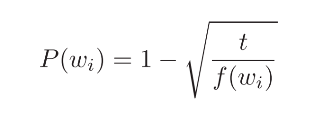
f(w_i) is the frequency of word w_i and t is a chosen threshold, typically around 10^-5.