Can you trust the trend? Discovering Simpson’s paradoxes in social data Alipourfard et al., WSDM’18
In ‘Same stats, different graphs,’ we saw some compelling examples of how summary statistics can hide important underlying patterns in data. Today’s paper choice shows how you can detect instances of Simpson’s paradox, thus revealing the presence of interesting subgroups, and hopefully avoid drawing the wrong conclusions. For the evaluation part of the work, the authors look at question-answering on Stack Exchange (Stack Overflow, for many readers of this blog I suspect).
We investigate how Simpson’s paradox affects analysis of trends in social data. According to the paradox, the trends observed in data that has been aggregated over an entire population may be different from, and even opposite to, those of the underlying subgroups.
Let’s jump straight to an example. In Stack Exchange someone posts a question and other users of the system post answers (ignoring the part about the question first being deemed worthy of the forum by the powers-that-be). Users can vote for answers that they find helpful, and the original poster of the question can accept one of the answers as the best one. What factors influence whether or not a particular answer is accepted as the best one? One of the variables that has been studied here is when in a user’s session an answer is posted. Suppose I’m feeling particularly helpful today, and I log onto to Stack Overflow and start answering questions to the best of my ability. I answer one question, then another, then another. Is my answer to the first question more or less likely to be accepted as a best answer than my answer to the third question? If we look at the data from 9.6M Stack Exchange questions, we see the following trend:

It seems that the more questions I’ve previously answered in a given session, the greater the probability my next answer will be accepted as the best one! That seems a bit odd. Do question answerers get into the flow? Do they start picking ‘easier’ questions (for them) as the session goes on?
Here’s another plot of exactly the same dataset, but with the data disaggregated by session length. Each different coloured line represents a session of a different length (i.e., sessions where the user answered only one question, sessions where the user answered two questions, and so on).

When we compare sessions of the same length, we clearly see exactly the opposite trend: answers later in a session tend to fare worse than earlier ones! The truth is that “each successive answer posted during a session by a user on Stack Exchange is shorter, less well documented with external links and code, and less likely to be accepted by the asker as the best answer.”
When measuring how an outcome changes as a function of an independent variable, the characteristics of the population over which the trend is measured may change as a function of the independent variable due to survivor bias.
To illustrate, here’s an example of that Stack Exchange data broken down by session length. Note the massive class imbalances (many more sessions of length one than length eight for example).
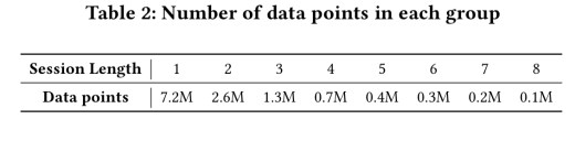
When calculating acceptance probability for the aggregate data, consider the case of computing the probability that the third answer in a session is accepted as the best one. Of the 12.8M total data points, 9.6M of them aren’t eligible to contribute to this analysis (sessions of length one or two). Thus there is a survivorship bias – when we get to the third answer, the first two have already failed to be accepted, indicating that perhaps the new answer is facing weaker competition. This increases the probability that the third answer will be accepted as the best. (And so on, as session lengths get longer and longer).
… despite accumulating evidence that Simpson’s paradox affects inference of trends in social and behavioral data, researchers do not routinely test for it in their studies.
Identifying Simpson’s paradoxes
We’d like to know if a Simpson’s paradox exists so that we don’t draw the wrong conclusions, and also because it normally suggests something interesting happening in the data: subgroups of the population which differ in their behaviour in ways which are significant enough to affect aggregate trends.
We propose a method to systematically uncover Simpson’s paradox for trends in data.
Let Y be the outcome being measured (e.g., the probability than an answer is accepted as the best one), and 


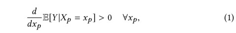
If
A trend in Y as a function of
And the reverse trend when conditioned on
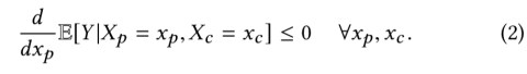
We’re looking for pairs where both equation (1) and (2) are true simultaneously. The process starts out by fitting linear models. Let the relationship between Y and
![\displaystyle \mathbb{E}[Y|X_p = x_p] = f_p(\alpha + \beta x_p)](https://s0.wp.com/latex.php?latex=%5Cdisplaystyle+%5Cmathbb%7BE%7D%5BY%7CX_p+%3D+x_p%5D+%3D+f_p%28%5Calpha+%2B+%5Cbeta+x_p%29&bg=eeeeee&fg=666666&s=0&c=20201002)
(Here 

We can use a similar linear model (with different values of alpha and beta) for the conditioned expectation:
![\displaystyle \mathbb{E}[Y|X_p = x_p, X_c = x_c] = f_{p,c}(\alpha (x_c) + \beta (x_c) x_p)](https://s0.wp.com/latex.php?latex=%5Cdisplaystyle+%5Cmathbb%7BE%7D%5BY%7CX_p+%3D+x_p%2C+X_c+%3D+x_c%5D+%3D+f_%7Bp%2Cc%7D%28%5Calpha+%28x_c%29+%2B+%5Cbeta+%28x_c%29+x_p%29&bg=eeeeee&fg=666666&s=0&c=20201002)
When fitting linear models
we have not only fitted a trend parameter
. From this, we have three possibilities:
By comparing the sign of
Although [our equations] state that the signs from the disaggregated curves should all be different from the aggregrated curve, in practice this is too strict, especially as human behavioral data is noisy. Thus, we compare the sign of the fit to aggregated data to the simple average of the signs of fits to disaggregated data.
Here’s the algorithm pseudocode:

Using the Stack Exchange data, the authors used this algorithm to find several instances of Simpson’s paradox:
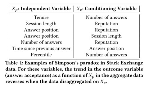
We looked at one of these earlier. Here’s a breakdown of the paradox regarding acceptance probability versus the total number of answers posted by a user in their account lifetime.

An analysis of the mathematical formulation of Simpson’s paradox presented above also reveals two necessary conditions for a paradox to arise:
- The distribution of the conditioning variable
- The expectation of
, conditioned on
The last word
Since social data is often generated by a mixture of subgroups, existence of Simpson’s paradox suggests that these subgroups differ systematically and significantly in their behavior. By isolating important subgroups in social data, our method can yield insights into their behaviors.

I think you misinterpreted the plots. The plots show the answer position not the session length. Your discussion of the plots seems to assume that the plots show session length.
The disaggregated plot shows a line for sessions of various lengths, then the x axis is answer position within that session, so it includes both. However I think the sentence starting “Thus there is a survivorship bias – when we get to the third answer, the first two have already failed to be accepted…” is incorrect, earlier answers in a session were not necessarily rejected, and anyway they were answers to different questions.
For example, following the first plot which shows Acceptance Probability vs Answer Position, is the sentence “It seems that the more questions I’ve previously answered in a given session, the greater the probability my next answer will be accepted as the best one!”. However, the way I understand the plot is that the more unaccepted answers there are for a question the higher the probability that your answer will be accepted if you post it.
From the paper “Answer position: Index of the answer within a session.” So it’s not the answer position within the set of answers for a single question. Each answer in the session will be for a different question.
Thanks James, I was wrong. I am off to my reading comprehension class.
I agree with James, the whole paragraph “when we get to the third answer, the first two have already failed to be accepted, indicating that perhaps the new answer is facing weaker competition. This increases the probability that the third answer will be accepted as the best” looks very strange, I suspect it is either incorrect, or formulated in a very confusing way.