Automatic database management system tuning through large-scale machine learning Aken et al. , SIGMOD’17
Achieving good performance in DBMSs is non-trivial as they are complex systems with many tunable options that control nearly all aspects of their runtime operation.
OtterTune uses machine learning informed by data gathered from previous tuning sessions to tune new DBMS deployments. In experiments with OLTP workloads (on MySQL and Postgres) and OLAP workloads (on Vector), OtterTune produces a DBMS configuration that achieves 58-94% lower latency compared to the default settings or configurations generated by other tuning advisors.
We also show that OtterTune generates configurations in under 60 minutes that are within 94% of ones created by expert DBAs.
Tuning challenges
The optimal configuration is different for every application / workload. (If this wasn’t true, presumably by now the default settings would be close to the optimal, which they aren’t!). To demonstrate this the authors take three different workloads and find an optimal configuration for each of them. Configuration 1 is the best for workload 1, and so on. Now see what happens when you run all three workloads under each configuration:
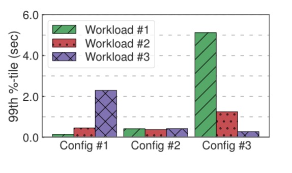
What’s best for one workload is very clearly not the best for the others!
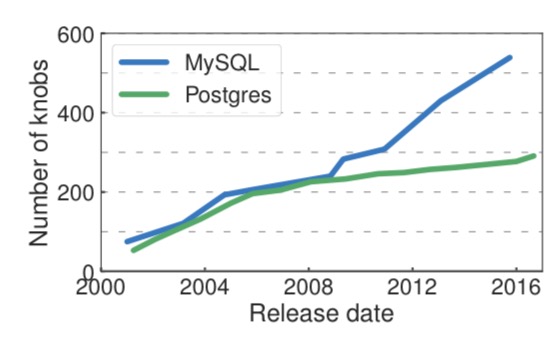
Furthermore, for any given workload, there are a lot of configuration parameters to play with. The following chart shows the growth in the number of configuration parameters (knobs) in MySQL and Postgres over time:
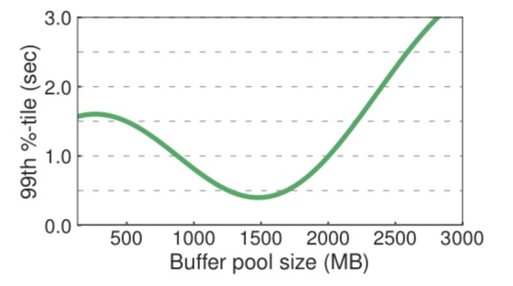
Each individual configuration parameter may have many possible settings, and the differences in performance from one setting to the next may not be regular. Here’s an illustration showing the relationship between MySQL’s buffer pool size and latency for one workload:
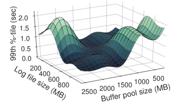
And if all that wasn’t complex enough, many of the parameters are inter-dependent such that changing one affects the others.
The different combinations of knob settings means that finding the optimal configuration is NP-hard.
Here’s an example showing the inter-dependencies between log file size and buffer pool size in MySQL for a workload:
How OtterTune works
OtterTune is a tuning service that works with any DBMS. It maintains a repository of data collected from previous tuning sessions, and uses this data to build models of how the DBMS responds to different knob configurations. For a new application, it uses these models to guide experimentation and recommend optimal settings. Each recommendation provides OtterTune with more information in a feedback loop that allows it to refine its models and improve their accuracy.
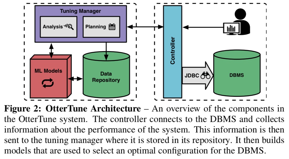
At the start of an tuning session the DBA specifies the metric to optimise (latency, throughput, …). OtterTune then connects to the DBMS and determines the hardware profile (just an identifier from a pre-defined list at the moment, e.g., an EC2 instance type) and current configuration. Then the target workload is run (either to completion, or for a fixed duration) while OtterTune observes the chosen optimisation metric. At the end of the run, OtterTune grabs all of the DBMS internal metrics (statistics and counters etc.). These are stored in the repository and OtterTune selects the next configuration to test. This happens in two phases:
- OtterTune tries to map the run to one it has seen (and tuned) in the past (workload characterization), giving a strong indication of where to look in the search space.
- Using this information OtterTune identifies and ranks the most important configuration parameters and settings to try.
This process of observing a run under a given configuration and selecting the next configuration to try based on the results continues until the DBA is satisfied with the improvement over the initial configuration. To help the DBA determine when to stop, OtterTune provides an estimate of how much better the recommended configuration is than the best seen so far.
OtterTune assumes that the physical design of the database (indices, materialized views etc.) is reasonable. Future work may investigate how to apply similar techniques to optimise the database’s physical design. (See also Peloton, which we looked at earlier this year).
OtterTunes’s machine learning pipeline
Let’s take a deeper look at OtterTune’s machine learning pipeline, which is where all the smarts take place.

Before OtterTune can characterise a workload, it first tries to discover a model that best represents its distinguishing aspects. This process uncovers the most important DBMS metrics and the most important configuration parameters for the workload. All of the internal metrics are collected, and then a combination of factor analysis and k-means clustering is used to find the most important ones. Factor analysis aims to find a smaller set of latent factors that explain (underlie) the observed variables (it’s related to PCA, but not the same). Each factor is a linear combination of the original variables, and factors can be ordered by the amount of variability in the original data they explain.
We found that only the initial factors are significant for our DBMS metric data, which means that most of the variability is captured by the first few factors.
The results of the factor analysis yield coefficients for metrics in each of the selected factors. From these coefficients closely correlated metrics can be identified and pruned. The remaining metrics are then clustered using the factor coefficients as coordinates. This results in clusters of metrics as shown in the following figure:
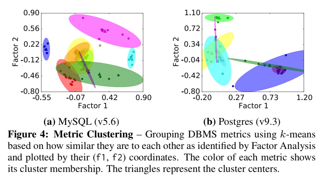
Inspecting the clusters shows that each cluster corresponds to a distinct aspect of a DBMS’s performance.
From each cluster, OtterTune keeps a single metric, the one closest to the cluster center.
From the original set of 131 metrics for MySQL and 57 for Postgres, we are able to reduce the number of metrics by 93% and 82%, respectively.
Having reduced the metric space, OtterTune next seeks to find the subset of configuration parameters which have the most impact on the target objective function (optimisation goal).
OtterTune uses a popular feature selection technique for linear regression, called Lasso, to expose the knobs that have the strongest correlation to the system’s overall performance. In order to detect nonlinear correlations and dependencies between knobs, we also include polynomial features in our regression.
The number of features that Lasso keeps depends on the strength of a penalty parameter that penalises models with large weights. By starting with a large penalty and gradually reducing it, it is possible to observe the order in which configuration parameters are added back into the regression, and this ordering is used to determine how much of an impact they have on the target metric.
The Lasso computations are performed in the background as new data arrives from different tuning sessions. Each invocation takes around 20 minutes and consumes about 10GB of memory for a repository with 100K trials and millions and data points.
From the ranked list, OtterTune dynamically increases the number of knobs used in a tuning session over time. “As we show in our evaluation, this always produces better configurations than any static knob count.”
To find the closest matching workload from those it has seen before, OtterTune computes the Euclidean distance between the vector of (non-redundant) metrics for the target workload and the corresponding vector for those in its repository. This matching is repeated after each experiment while OtterTune gathers more data since the matched workload can vary for the first few experiments before converging on a single workload.
To recommend a configuration to try next, OtterTune uses Gaussian Process (GP) regression. (We looked at Bayesian optimisation previously with CherryPick and BOAT).
OtterTune starts the recommendation step by reusing the data
from the workload that it selected previously to train a GP model.
It updates the model by adding in the metrics from the target workload that it has observed so far. But since the mapped workload is not exactly identical to the unknown one, the system does not fully trust the model’s predictions. We handle this by increasing the variance of the noise parameter for all points in the GP model that OtterTune has not tried yet for this tuning session.
Whether OtterTune chooses exploration (investigating areas in the model where its confidence is low) or exploitation (searching around configurations close to its best so far) depends on the variance of data points in its GP model. It will always choose the configuration with the greatest expected improvement.
OtterTune uses gradient descent to find the local optimum on the surface predicted by the GP model using a set of configurations, called the initialization set, as starting points.
The initialization set contains a mix of top performing configurations from the current tuning session, and configurations with randomly selected values. It takes OtterTune about 20 seconds to complete the gradient descent search per observation period.
Evaluation
OtterTune is evaluated using workloads from YCSB, TPC-C, a Wikipedia-based OLTP workload, and TPC-H and MySQL v5.6, Postgres v9.3, and Actian Vector v4.2.
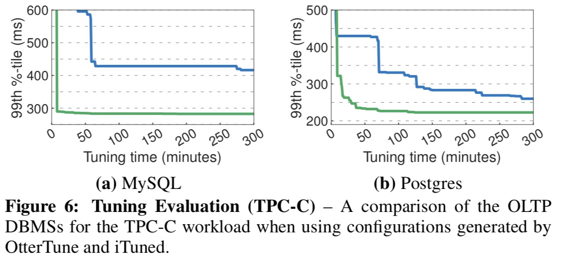
OtterTune is able to find good configurations within 15-60 minutes, as evidenced by the charts below (green line is OtterTune, the blue line is another tuning tool called iTuned).
The key charts for me though are the following, which show how effective the configurations found by OtterTune are when compared to (a) the DBMS default settings, (b) tuning scripts from open-source tuning advisor tools, (c) an experienced DBA, and (d) the configuration used by Amazon RDS.

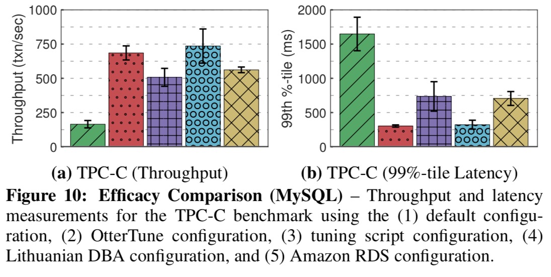
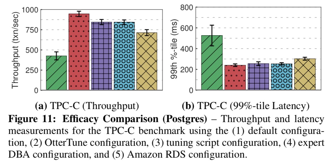
Our results show that OtterTune produces configurations that achieve up to 94% lower latency compared to [the DBMS] default settings or configurations generated by other tuning advisors. We also show that OtterTune generates configurations in under 60 minutes that are comparable to ones created by human experts.
Finally a “number of knobs” graph. I was just advising a colleague recently about twiddling avoidance.