Declarative recursive computation on an RDBMS… or, why you should use a database for distributed machine learing Jankov et al., VLDB’19
If you think about a system like Procella that’s combining transactional and analytic workloads on top of a cloud-native architecture, extensions to SQL for streaming, dataflow based materialized views (see e.g. Naiad, Noria, Multiverses, and also check out what Materialize are doing here), the ability to use SQL interfaces to query over semi-structured and unstructured data, and so on, then a picture begins to emerge of a unifying large-scale data platform with a SQL query engine on top that addresses all of the data needs of an organisation in a one-stop shop. Except there’s one glaring omission from that list: handling all of the machine learning use cases.
Machine learning inside a relational database has been done before, most notably in the form of MADlib, which was integrated into Greenplum during my time at Pivotal. The Apache MADLib project is still going strong, and the recent (July 2019) 1.16 release even includes some support for deep learning.
To make that vision of a one-stop shop for all of an organisation’s data needs come true, we need to be able to handle the most demanding large scale machine learning tasks – those requiring distributed learning. Today’s paper choice, subtitled “Why you should use a database for distributed machine learning” seeks to fill that gap. It would be a bold departure from the current imperative high-level DSL based approach to deep learning taken by TensorFlow et al., but at the same time it also offers some compelling looking advantages. Even in deep learning, do all roads eventually lead back to SQL??
We consider how to make a very small set of changes to a modern relational database management system (RDBMS) to make it suitable for distributed learning computation… We also show that there are key advantages to using an RDBMS as a machine learning platform.
Why would anyone want to do that???
Why would anyone want to run deep learning computations within an RDBMS??
On the one hand, because current deep learning approaches to distribution can only go so far just with data parallelism based-approaches (one model, split up the data), and instead are pushing into model-parallelism to get to the next level (split up the model itself across multiple nodes).
The distributed key-value stores (known as parameter servers) favored by most existing Big Data ML systems (such as TensorFlow and Petuum) make it difficult to build model parallel computations, even “by hand”.
On the other hand, by switching to a relational model of computation, model parallelism looks pretty similar to data parallelism, and we can take advantage of heavily optimised distributed database engines. SQL provides a declarative programming interface, below which the system itself can figure out the most effective execution plans based on data size and statistics, layout, compute hardware etc..
Be careful what you ask for (materialize)
If we assume an RDBMS ‘lightly augmented’ to handle matrix and vector data types, such as SimSQL then we’re actually not far away from being able to express machine learning computations in SQL today.
Given a weights table W storing chunks of the weights matrix, and an activations table A storing activations, and an AEW table storing the values needed to compute weights for the next iteration, then we can express the backward pass of iteration i of a feed-forward machine learning model with eight hidden layers in SQL.
W (ITER, LAYER, ROW, COL, MAT)
A (ITER, LAYER, COL, ACT)
AEW (LAYER, ROW, COL, ACT, ERR, MAT)
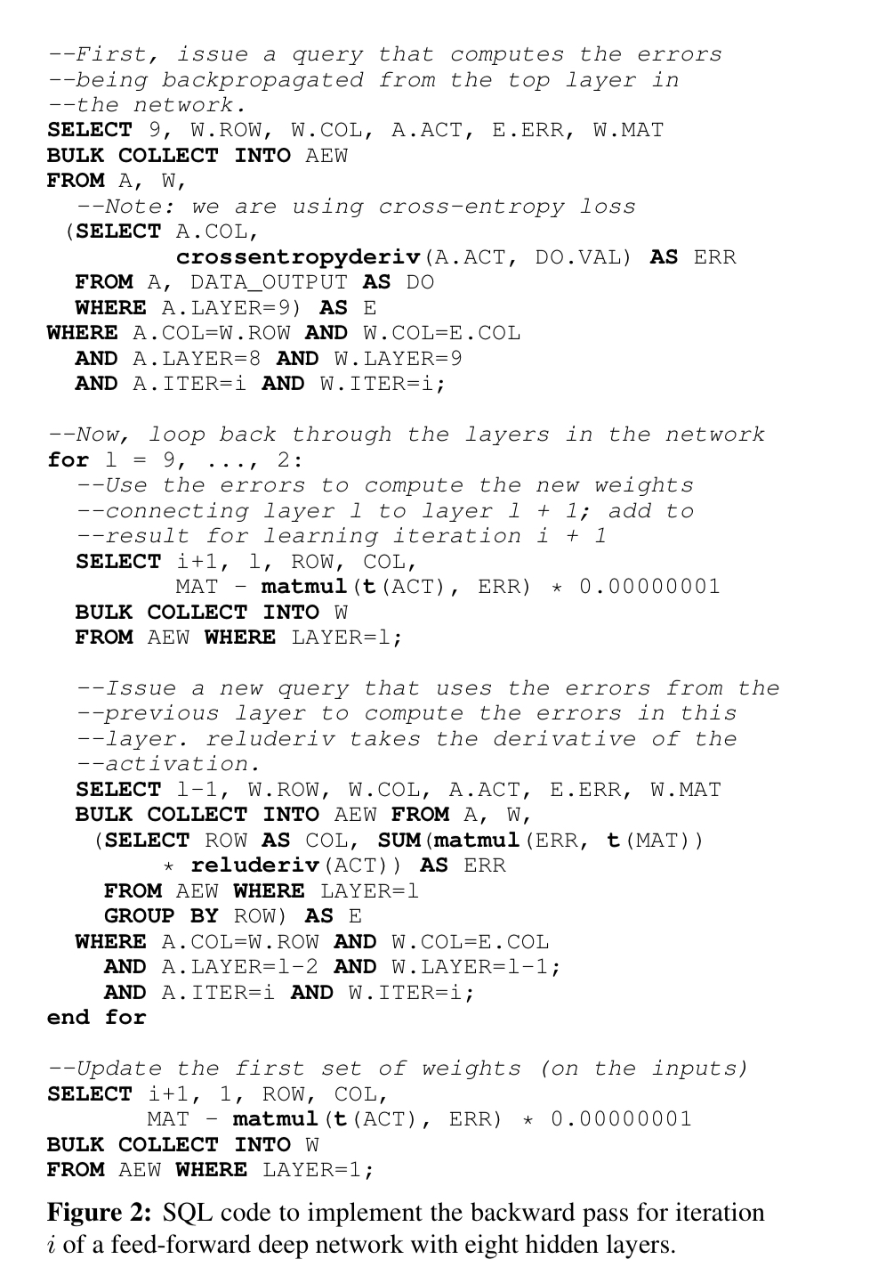
Aside from the fact that this doesn’t look very pretty (cf. MLP in MADLib), it’s also quite imperative for SQL (note the for loop). The problem caused by that is the AEW table used to materialize the state passed between iterations: that state can grow very large very quickly. We’d like to get rid of the imperative for-loop so that we can implement pipelining behind a declarative query expression.
Recursive SQL extensions
Classic SQL already has recursion support through something called “Common Table Expressions.” Here we want something a little different to that, essentially the ability to express lazy materialization over arbitrarily large sequences of tables.
The authors introduce the notion of multiple versions of a table accessed via array-style indices, using Pascal’s triangle as an example.
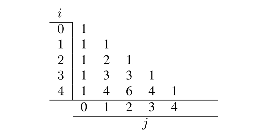
Given a base table, e.g.
CREATE TABLE pascalsTri[0][0] (val) AS
  SELECT val FROM VALUES (1);
Then we can define additional versions recursively, e.g. for the diagonals of Pascal’s triangle (j = i):
CREATE TABLE pascalsTri[i:1...][i] (val) AS
  SELECT * FROM pascalsTri[i-1][i-1];
For the cases where j = 0:
CREATE TABLE pascalsTri[i:1...][0] (val) AS
  SELECT * FROM pascalsTri[i-1][0];
And for everything else:
CREATE TABLE pascalsTri[i:2...][j:1...i-1] (val) AS
  SELECT pt1.val + pt2.val AS val
  FROM pascalsTri[i-1][j-1] AS pt1,
       pascalsTri[i-1][j] AS pt2;
So that later on we can issue a query such as SELECT * FROM pascalsTri[56][23] and the system will unwind the recursion to express the required computation as a single relational algebra statement.
The EXECUTE keyword allows queries over multiple versions of a table at the same time. For example:
EXECUTE (
  FOR j in 0...50:
    SELECT * FROM pascalsTri[50][j]);
We can also request that a table be explicitly materialized using the MATERIALIZE keyword (for dynamic programming), and we can merge multiple recursively defined tables using UNION.
Recursive learning in SQL
Armed with these new extensions we can define a forward pass computation (computing the level of activation of the neurons at each layer) like this:
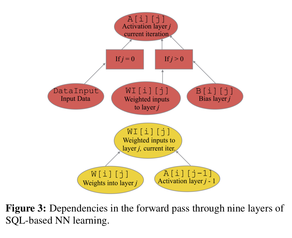
-- First layer of activations
CREATE TABLE A[i:0...][j:0] (COL, ACT) AS
  SELECT DI.COL, DI.VAL
  FROM DATA_INPUT AS DI;

-- Propagating activations
CREATE TABLE WI[i:0...][j:1...9] (COL, VAL) AS
  SELECT W.COL, SUM(matmul(A.ACT, W.MAT))
  FROM W[i][j] AS w, A[i][j-1] AS A
  WHERE W.ROW = A.COL
  GROUP BY W.COL;

-- Subsequent activations
CREATE TABLE A[i:0...][j:1...8] (COL,ACT) AS
  SELECT WI.COL, relu(WI.VAL + B.VEC)
  FROM WI[i][j] AS WI, B[i][j] AS B
  WHERE WI.COL = B.COL;

-- Prediction
CREATE TABLE A[i:0...][j:9] (COL, ACT) AS
  SELECT WI.COL, softmax(WI.VAL + B.VEC)
  FROM WI[i][j] AS WI, B[i][j] AS B
  WHERE WI.COL = B.COL;
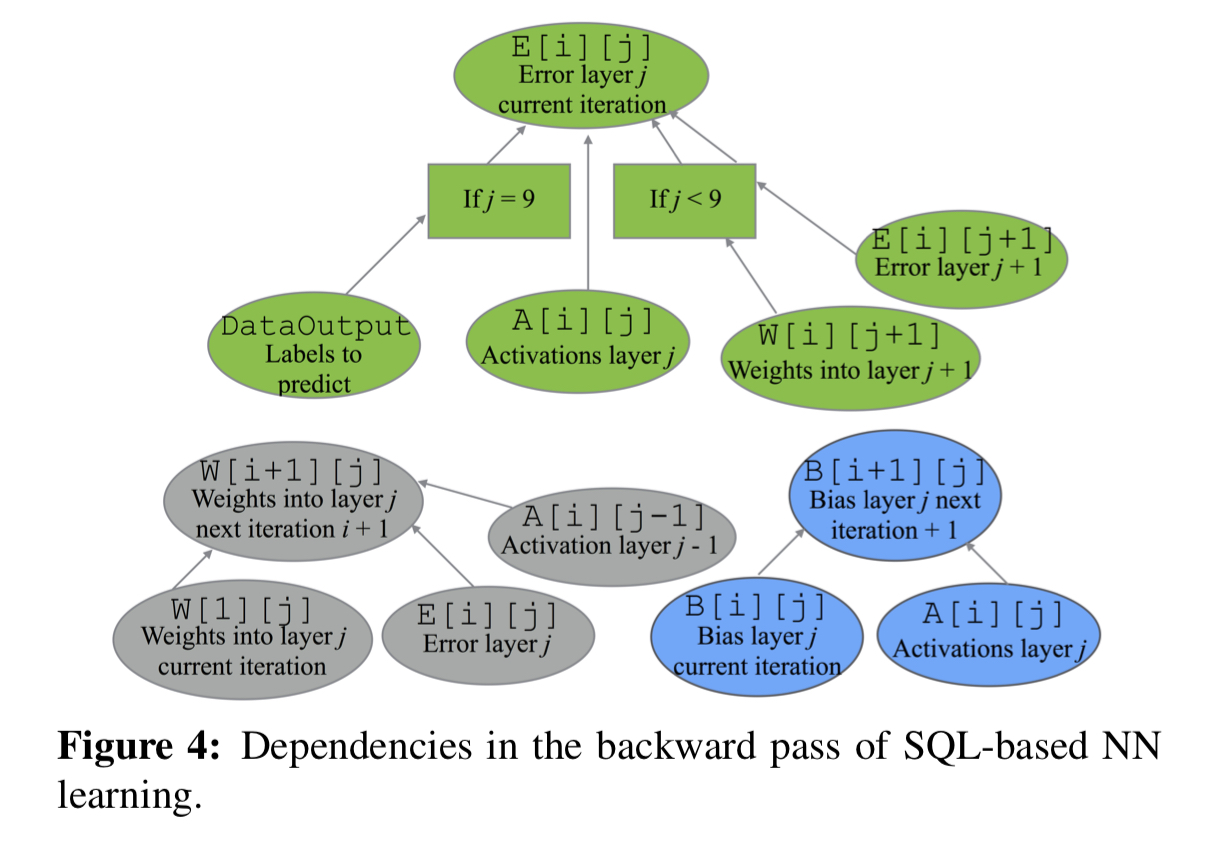
The backward pass can be expressed similarly:
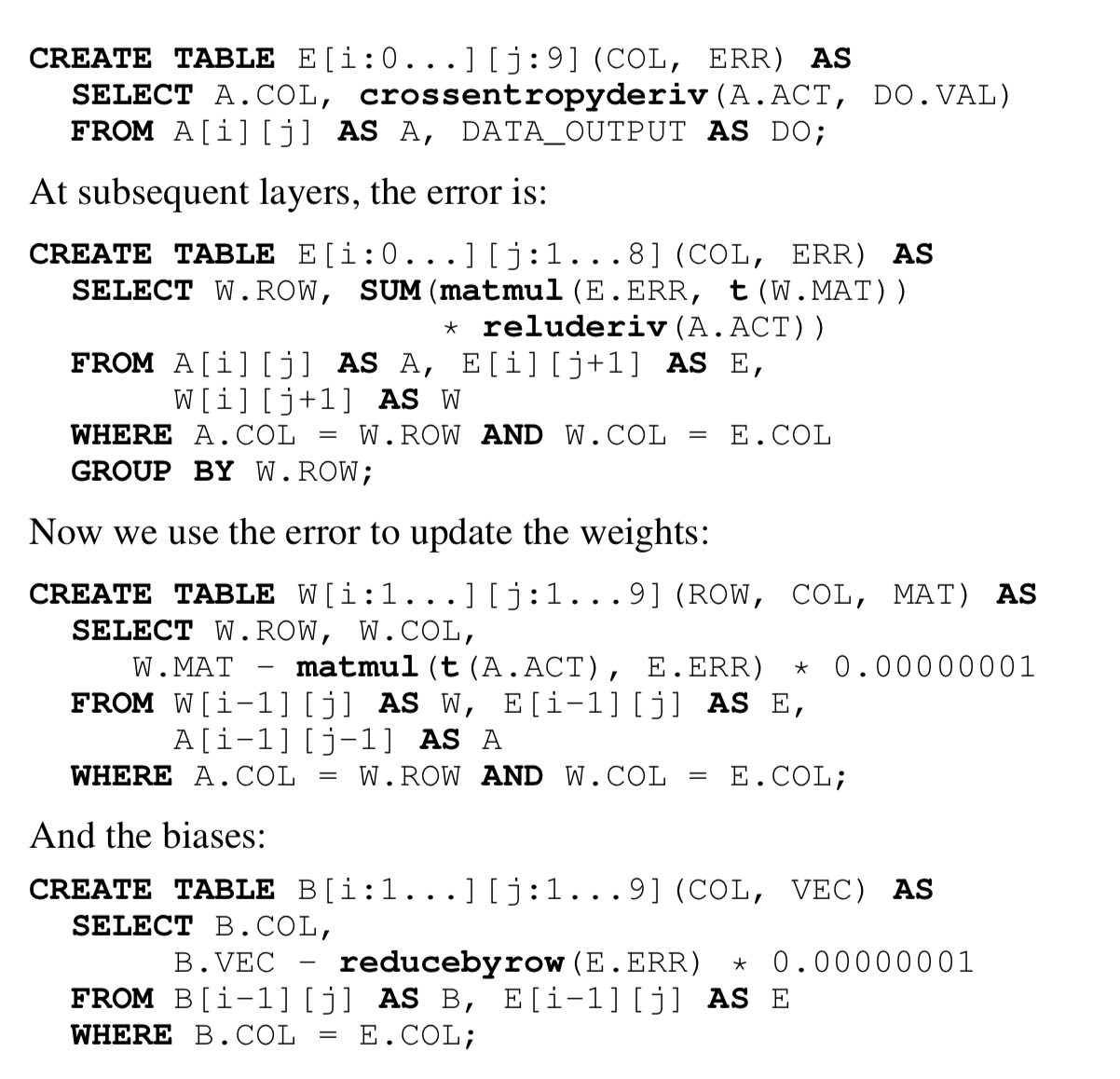
Execution planning for efficiency
The paper goes into quite some detail on how the large and complex computations implied by SQL specifications of ML workloads can be efficiently compiled and executed by an RDBMS. Here I’ll just touch on the highlights.
From the query, we can unroll the recursion to create a single, un-optimised relational algebra plan (DAG). The next step is to chop that plan up into pieces, with each sub-plan being called a frame. Clearly the chosen decomposition can have a big impact on the resulting query performance. If we go too granular we might lose the opportunity to find good optimisations within a frame (e.g., optimal join orderings). So frames have a minimum size. The next major consideration is the amount of inter-frame communication required by a given decomposition. A good approximation for the this is the number of pipeline breakers introduced.
A pipeline breaker occurs when the output of one operator must be materialized to disk or transferred over the network, as opposed to being directly communicated from operator to operator via CPU cache, or, in the worst case, via RAM. An induced pipeline breaker is one that would not have been present in an optimal physical plan but was forced by the cut.
Even figuring out whether a given cut will introduce a pipeline breaker is not straightforward, but can be estimated probabilistically. This cost feeds into an overall optimisation to find the best plan decomposition, as an instance of the well-known generalized quadratic assignment problem (GQAP). One of things that’s well-known about GQAP is that it’s a very hard problem! You can probably guess what’s coming next…. a greedy approximation.
Starting from one source operator, we greedily add operators to the frame, selecting the one that yields the smallest increase in frame cost, until the frame size exceeds a minimum threshold. The results are dependent on the initial source node you happened to pick, but this can be remedied by running the greedy algorithm once for every possibly starting operation.
Experimental results
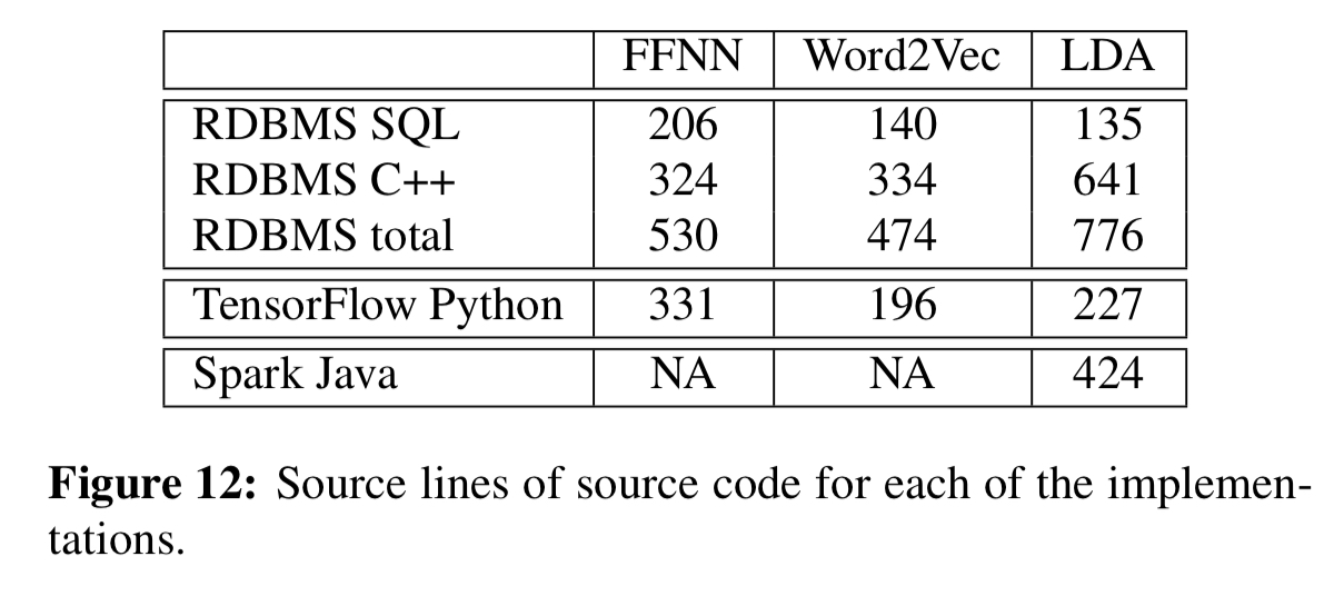
The evaluation compares distributed implementations of a multi-layer feed-forward neural network (FFNN), the Word2Vec algorithm, and a distributed collapsed Gibbs sampler for LDA. The implementations require both SQL and also some UDFs written in C++. The table below shows representative line counts as compared to TensorFlow and Spark. Once a library of UDFs have been built up of course, they could be reused across computations.
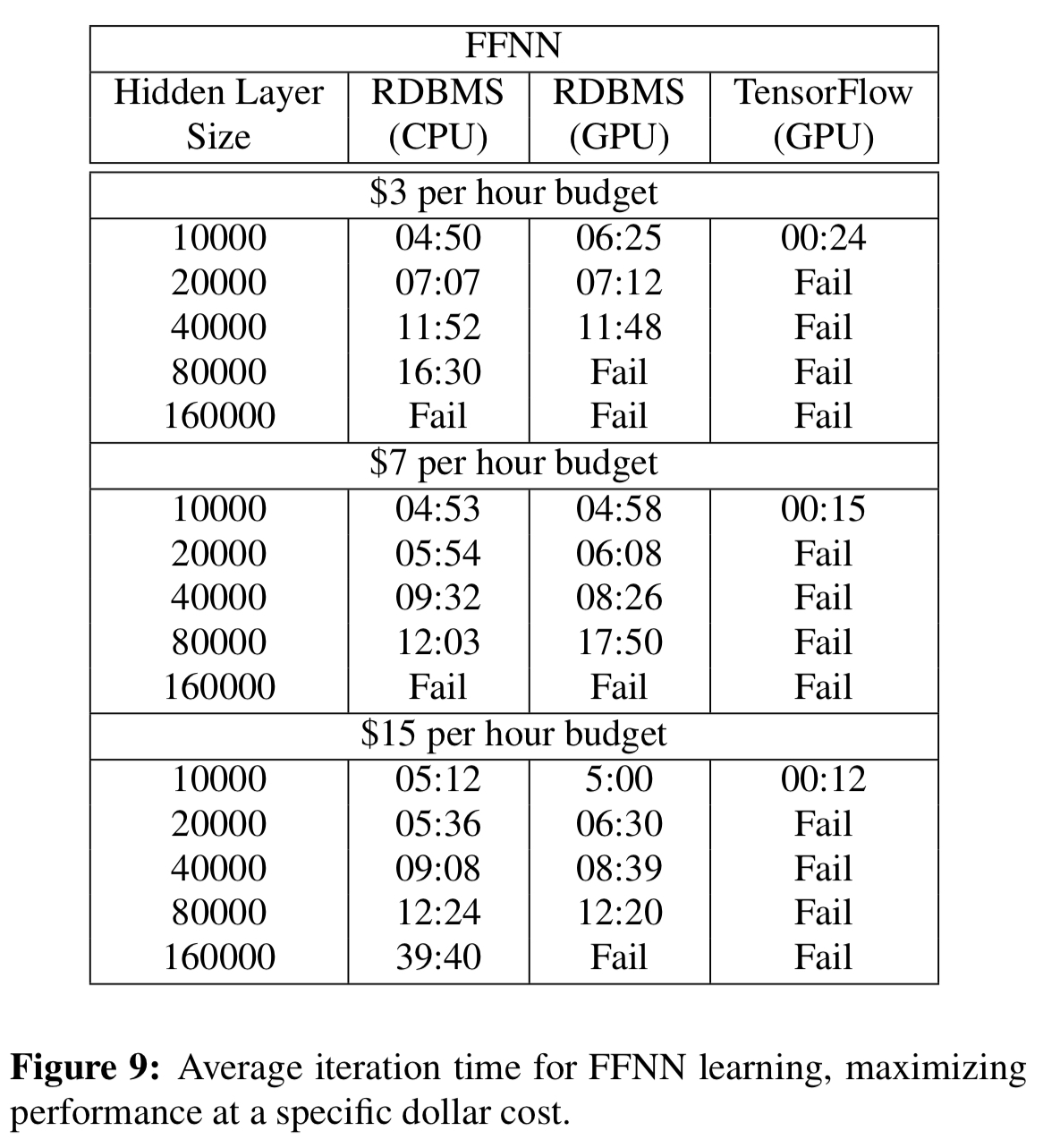
For the feed-forward neural network, TensorFlow using GPUs is still significantly faster with smaller hidden layers, but cannot scale. Beyond that, the RDBMS wins:
For the Word2Vec and LDA computations the speed-ups as the number of dimensions/topics grows are very significant (e.g 8.5 minutes vs almost 5hrs for LDA with 50,000 topics).
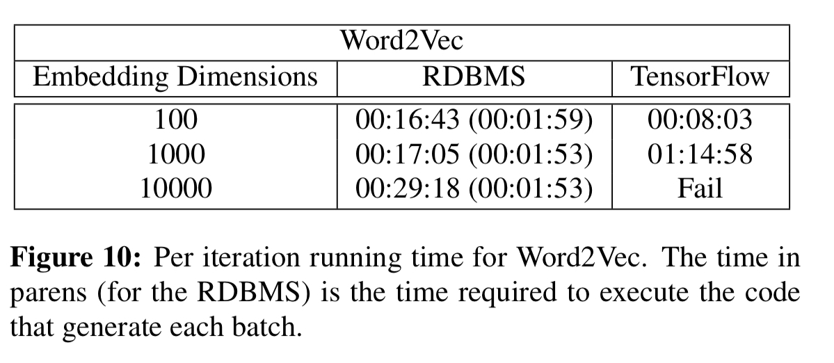
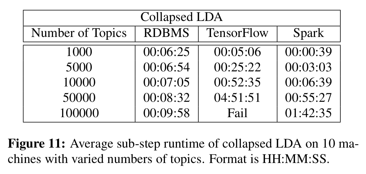
We have shown that model parallel, RDBMS-based ML computations scale well compared to TensorFlow, and that for Word2Vec and LDA, the RDMBS-based computations can be faster than TensorFlow. The RDBMS was slower than TensorFlow for GPU-based implementations of neural networks, however. Though some of this discrepancy was due to the fact that we implemented our ideas on top of a research prototype, high-latency Java/Hadoop system, reducing that gap is an attractive target for future work.
Machine learing, I suspect a typo. Or an “interesting” technological advance.