Robust learning from untrusted sources Konstantinov & Lampert, ICML’19
Welcome back to a new term of The Morning Paper! Just before the break we were looking at selected papers from ICML’19, including “Data Shapley.” I’m going to pick things up pretty much where we left off with a few more ICML papers…
Data Shapley provides us with one way of finding and correcting or eliminating low-value (and potentially harmful) data points from a training set. In today’s paper choice, Konstantinov & Lampert provide a way of assessing the value of datasets as a whole. The idea is that you might be learning e.g. a classifier by combining data from multiple sources. By assigning a value (weighting) to each of those data sources we can intelligently combine them to get the best possible performance out of the resulting trained model. So if you need more data in order to improve the performance of your model, ‘Robust learning from untrusted sources’ provides an approach that lets you tap into additional, potentially noisier, sources.
It’s similar in spirit to Snorkel which we looked at last year, and is designed to let you incorporate data from multiple ‘weakly supervised’ (i.e. noisy) data sources. Snorkel replaces labels with probability-weighted labels, and then trains the final classifier using those.
The big idea
You have at least one data source that you trust to have reasonable quality, which we’ll call the reference dataset. In addition you have N further data sources available, of varying quality.
Two extremes of learning from all this data are to (a) use only the known high quality reference data source, discarding the others, and (b) train using all the available data regardless of quality. The goal of this paper is to find a middle-ground that lets us makes use of all of the data available, without dragging the resulting model performance down due to noisy data.
… we propose a method that automatically assigns weights to the sources… the weights are assigned to the sources according to the quality and reliability of the data they provide, quantified by an appropriate measure of trust we introduce. This is achieved by comparing the data from each source to a small reference dataset, obtained or trusted by the learner.
In the evaluation, the resulting models consistently outperform models trained on either the reference dataset only, or all of the datasets, for any amount and type of data contamination considered in the study.
How good is that data source?
Intuitively, a good learning algorithm will assign more weight to sources whose distribution is similar to the target one, and less weight to those that provide different or low-quality data.
The phrase ‘similar to the target one’ implies we’re going to need a distance measure over distributions so that we can compare them. For this use case, the ideal distance measure would be one that gives us a strong correlation with the performance of a learned classifier. Now, there’s nothing that correlates better with the performance of a learned classifier than… the performance of a learned classifier!
The discrepancy between the distribution of a given dataset and the reference dataset
is defined to be the difference in the expected loss of a predictor trained on the reference dataset and a predictor trained on the additional dataset.
Intuitively, the discrepancy between the two distributions is large, if there exists a predictor that performs well on one of them and badly on the other. On the other hand, if all functions in the hypothesis class perform similarly on both, then
and
have low discrepancy.
Combining data sources
At this point we have a collection of datasets, and an indication of how ‘good’ each of those datasets is for the task in hand. Since we have a collection of trained classifiers, one per dataset, my intuition would be to use them as an ensemble and use weighted voting to combine their outputs. The natural first thing I would try is to have the weighting inversely proportional to the discrepancy score. That’s sort of what happens here, but the authors have a fancier way of determining the weights.
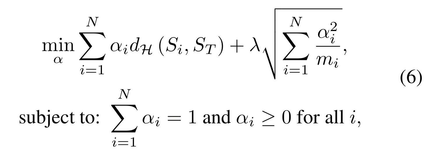
The weights are chosen by minimising the following objective function:
Let’s pick that apart a little bit…
- We have
different datasets to combine
is the weight assigned to the ith dataset
is the discrepancy score between dataset
and the reference dataset
.
The first term therefore is learning weights based directly on the discrepancy score. The constraint that the learned weights must sum to 1 prevents the algorithm simply assigning a very low or zero weight to each source.
The second term is a kind of regularisation parameter. is the number of data points in the ith dataset, so it’s designed to encourage more confidence to be placed in the result of classifiers trained over larger datasets.
Note that the first term is small whenever large weights are paired with small discrepancies and hence encourages trusting sources that provide data similar to the reference target sample. The second term is small whenever the weights are distributed proportionally to the number of samples per source. Thus, it acts as a form of regularization, by encouraging the usage of information from as many sources as possible.
is a hyperparameter controlling the balance between the two.
Incorporating private data
If one or more of the data sources is private or has constraints (e.g., it can’t be moved to the location where the training is taking place) then it can still be incorporated into the overall process. If the reference (target) dataset can be moved to the location of the private data, then the discrepancy score can be calculated locally there. If the reference dataset also cannot be shared, then it turns out it is still possible to compute empirical discrepancies without observing the data from the source directly. This works because the equation for determining discrepancy breaks down into two independent terms, one concerning the reference dataset, and one concerning the comparison dataset:
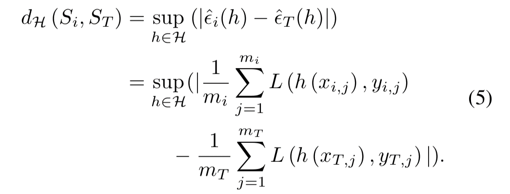
Therefore, each discrepancy can be estimated by using a sequence of queries to the source about the gradient of a minibatch from its data with respect to a current candidate for the predictor…
Evaluation
The first part of the evaluation is done using an Amazon products dataset with customer reviews for 957 Amazon products. The task is to learn a classifier per product which can classify reviews for that product as either positive or negative. The experiment focuses in on reviews for books, and provides to the learning algorithm a dataset based on reviews for the book in question, together with data from reviews of other books, and data from reviews of other non-book products. Each run ends up with 10 data sources to combine: 600 reviews from the target book, and 100 labelled reviews from 9 other products, varying , the number of these other products that are not books.
Intuitively, when learning to classify book reviews and given access to reviews from both some books and some non-books, a good learning algorithm will be able to leverage all this information, while being robust to the potentially misleading data coming from the less relevant products.
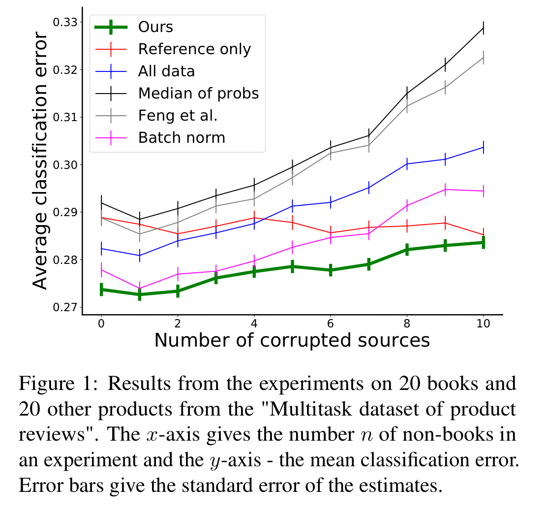
The resulting classifiers give much better results than either of the two extremes of (a) using only the reference dataset, and (b) just lumping all the data together in one unweighted pool.
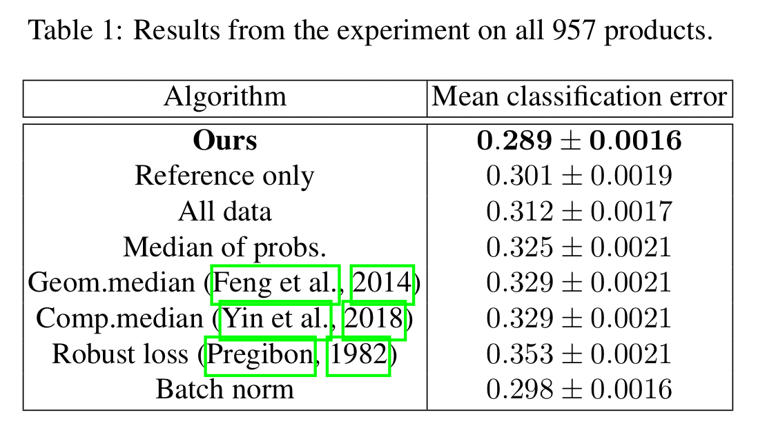
A variation on this looked across all 957 products, giving each classifier 100 reviews from its own dataset, and an additional set of 100 labelled reviews from every other product.
The second part of the evaluation uses the ‘Animals with Attributes 2’ dataset with 37,322 images of 50 different animal classes. A sample is taken of clean data to form the reference dataset, and then corrupted additional datasets are created using a variety of manipulations:
- Introducing label bias by setting labels of all corrupted samples to class 1
- Shuffling labels
- Shuffling features
- Blurring images
- Introducing dead pixels (for 30% of the image)
- Swapping RGB channels
For a given combination of target attribute, corruption strategy, and blend of true and corrupted datasets, the learning experiment is repeated 100 times.
The following table summarises the results over 85 different prediction tasks:
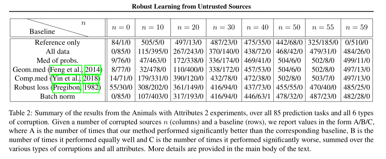
The results in table 2 show that our method performs significantly better than all baselines for many types of corruption and many values of n, especially for high levels of contamination, while essentially never performing significantly worse than any baseline.
15 thoughts on “Robust learning from untrusted sources”
Comments are closed.