Meta-learning neural bloom filters Rae et al., ICML’19

Bloom filters are wonderful things, enabling us to quickly ask whether a given set could possibly contain a certain value. They produce this answer while using minimal space and offering O(1) inserts and lookups. It’s no wonder Bloom filters and their derivatives (the family of approximate set membership algorithms) are used everywhere. Hash functions are the key to so many great algorithms, and Bloom filters are one of my favourite applications of them.

But Rae et al. think we can do even better, especially when it comes to the space required by an approximate set membership data structure. Being an ICLR paper of course, you won’t be surprised to learn that the solution involves neural networks. This puts us in the same territory as SageDB and ‘The case for learned index structures.’ Probably my favourite sentence in the whole paper is this one, which crisply sets out where machine learning might be able to find an advantage over traditional algorithms:

We build upon the recently growing literature on using neural networks to replace algorithms that are configured by heuristics, or do not take advantage of the data distribution.

Bloom filters are an example of an algorithm that doesn’t take advantage of the data distribution (in fact, most of the interesting variants introduce mechanisms to cope with the fact that the distribution isn’t always uniform, as opposed to exploiting the non-uniformity. See e.g. counting quotient filters).

The point about algorithms configured by heuristics is well made too, but hey, people with lots of hyperparameters shouldn’t throw stones ;)!

You’ve only got one shot

The setting for Neural Bloom Filters assumes a stream-like environment where you only get to see an input added to the set once. You see new data values as they arrive, and you need to do one-shot learning to remember their set-membership status. (With traditional Bloom filters this is the moment where we compute the hashes and OR them).

Instead of learning from scratch, we draw inspiration from the few-shot leaning advances obtained by meta-learning memory-augmented neural networks. In this setup, tasks are sampled from a common distribution and a network learns to specialize to (learn) a given task with few examples. This matches very well to applications where many Bloom Filters are instantiated over different subsets of a common data distribution.

For example, a Google Bigtable database usually contains one Bloom Filter per SSTable file. With a large table holding Petabytes of data that could mean 100,000 or more separate filters, all sharing a common row-key format and query distribution. So what we can do is periodically learn a base model offline, and then specialise it online for each of those filter instances.

Neural Bloom Filters

We can think of the array of bits used by a Bloom filter to test for membership as its memory, and the hash functions used by a Bloom filter as a way of addressing that memory. Neural Bloom filters also have memory and an addressing scheme, but things are a little more complicated…

Previous works such as the Neural Turing Machine and MemoryNetworks have explored augmenting networks with an external memory and a differentiable content-based addressing scheme. More recently, the Kanerva Machine introduced a level of indirection with a learnable addressing matrix that learns where to write. Neural Bloom filters are inspired by this scheme.

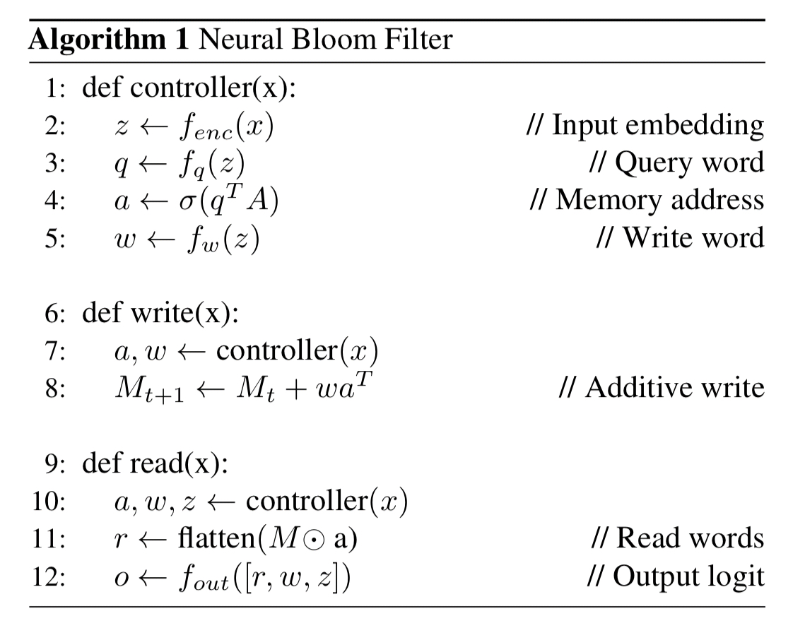
The overall Neural Bloom Filter architecture looks like this:

• A controller network encodes the input (which might be a row in a table, but could equally be e.g. an image) into an embedding . For image inputs the authors use a 3-layer CNN for this purpose, and for textual inputs a 128-hidden-unit LSTM.
• Two further networks learn to turn the representation into a word to be written to memory, , and a query which we’ll use to help figure out where to write to. The evaluation uses MLPs with a single hidden layer of size 128 for these networks.
• The query is combined with a learnable address matrix to yield the address to write to ( ).
• To have the network remember a new entry in the set, an additive write updates the memory by setting equal to .
• To test for membership (read), we component-wise multiply the obtained address with to obtain a read-word . The read word is fed into another MLP, together with and , and the output is project to a single scalar logit, representing the probability that the original input is a member of the set.

(I did warn you things were a little more complicated!)

As a Bloom filter replacement we’re still not done yet though. Bloom filters have a very important guarantee that if “filter says no” then we know that a given element is not in the set (no false negatives). The Neural Bloom Filter doesn’t give us that, just a probability that a given element is in the set. So we have to borrow a trick from ‘The case for learned index structures’ to deal with that. A threshold probability is used to determine when the filter will say yes, which means we might have some false negatives for elements we know to be in the set, but fall below the threshold. We keep track of these in a (much smaller) secondary Bloom filter (the plain-old data structure – PODS¹?- version). So the full look-up process becomes:

1. If the Neural Bloom Filter predicts membership with probability greater than the chosen threshold, return “(might be a) member”
2. Otherwise check the secondary Bloom filter, if it indicates the element might be a member, return “(might be a) member”
3. Otherwise return “not a member”

Evaluation

Our experiments explore scenarios where set membership can be learned in one-shot with improved compression over the classical Bloom filter.

The Neural Bloom Filter is compared against an LSTM, Differentiable Neural Computer (evolution of the Neural Turing Machine), Memory Network, and a PODS Bloom Filter. The main evaluation compares the space (in bits) of the model’s memory to a PODS Bloom Filter at a given false positive rate. The size computation for the models includes the state of the supplementary Bloom Filter needed to keep out false negatives.

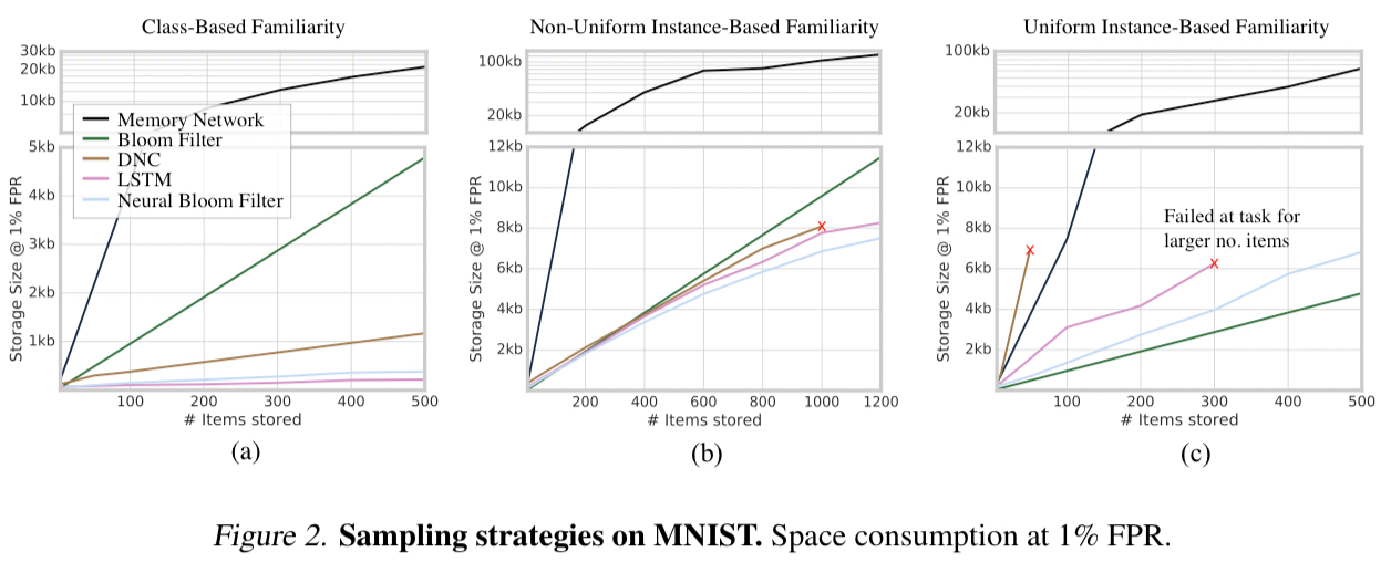
The first comparisons use MNIST images as the inputs, with three different set compositions:

1. Class-based familiarity: A highly structured task where each set of images comes from the same randomly selected class (e.g., they’re all 3s).
2. Non-uniform instance-based familiarity: A non-uniform task where images are sampled without replacement from an exponential distribution, and
3. Uniform instance-based familiarity: A completely unstructured task where each subset contains images sampled uniformly without replacement

We can see from the following figure that the Neural Bloom Filter uses significantly less space than a traditional Bloom Filter in the first two tasks where it has some structure to exploit, but fares worse than the traditional Bloom Filter in the third case where there is no such structure.

The overall conclusion from these sets of experiments is that the classical Bloom Filter works best when there is no structure to the data, however when there is (e.g. skewed data, or highly dependent sets that share common attributes) we do see significant space savings.

(Significant here can be an order-of-magnitude).

There’s an interesting experiment in section 5.3 of the paper where the authors play with different read and write operations and show that with small changes to them a Neural Bloom Filter can learn different algorithmic solutions. I don’t have space to cover it here, so please see the full paper if you’re interested in understanding how those operations influence results in a little more detail.

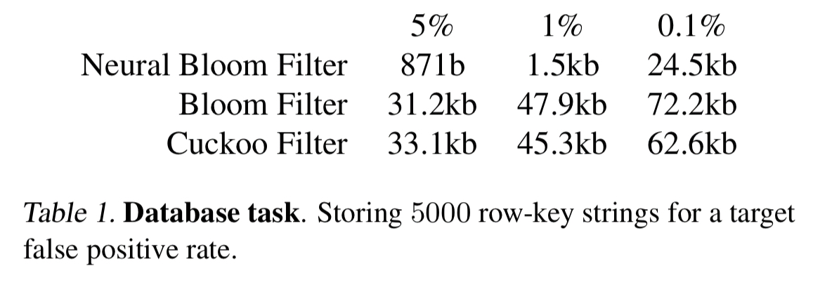
The authors also used compared Neural Bloom Filters against a PODS Bloom Filter and a Cuckoo Filter when indexing Bigtable tables (storing sorted string sets of size 5000, for a typical shard size when stored values are around 10kB). Neural Bloom Filters show a significant space saving of 3-40x, depending on the target false positive rate.

There’s an important catch though: on a CPU, Neural Bloom Filter lookups are about 400x slower than a PODS Bloom Filter lookup. If you can do multiple queries in parallel exploiting GPUs, then Neural Bloom Filters can claw some of that time back. Under high query loads therefore, Neural Bloom Filters could potentially be deployed “without a catastrophic decrease in throughput, if GPU devices are available” (emphasis mine). Given a GPU, the insertion throughput of a Neural Bloom Filter can outperform a PODS Bloom Filter.

Wrapping up

The Neural Bloom Filter relies on settings where we have an off-line dataset (both of stored elements and queries) that we can meta-learn over. In the case of a large database we think this is warranted, a database with 100K separate set membership data structures will benefit from a single (or periodic) meta-learning training routine that can run on a single machine and sample from the currently stored data, generating a large number of efficient data-structures. We envisage the space cost of the network to be amortized by sharing it across many neural Bloom Filters, and the timecost of executing the network to be offset by the continuous acceleration of dense linear algebra on modern hardware, and the ability to batch writes and queries efficiently.

To go ahead and introduce Neural Bloom Filters into your system you’ve got to really want those space savings. Just think about the comprehension, implementation, and trouble-shooting complexity here compared to plain old Bloom filters! It feels like it’s only a matter of time though, in one form or another the neural networks are coming…!!