Neural Turing Machines – Graves et al. 2014 (Google DeepMind)

A Neural Turing Machine is a Neural Network extended with a working memory, which as we’ll see, gives it very impressive learning abilities.

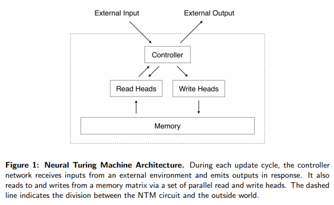
A Neural Turing Machine (NTM) architecture contains two basic components: a neural network controller and a memory bank. Like most neural networks, the controller interacts with the external world via input and output vectors. Unlike a standard network, it also interacts with a memory matrix using selective read and write operations. By analogy to the Turing machine we refer to then etwork outputs that parametrise these operations as “heads.”

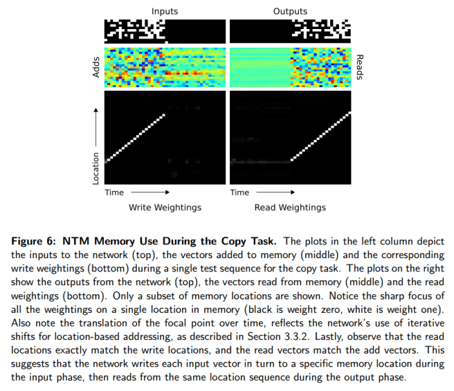
If a neural network has been likened to a brain, then this is like giving the brain a working memory. The network itself learns how best to use its memory when learning a solution to a given problem. An NTM trained on a copy task where the goal was to output a copy of an input sequence, learned a copy algorithm. By analysing the network and the interaction between the controller and the memory, the authors deduce that the sequence of operations performed by the network matches the following pseudocode:

initialise: move head to start location
while input delimiter not seen do
    receive input vector
    write input to head location
    increment head location by 1
end while
return head to start location
while true do
    read output vector from head location
    emit output
    increment head location by 1
end while

This is not something the authors programmed into the NTM, the NTM figured it out for itself, based on simply observing the inputs and desired outputs!

As I mentioned last week, the team at Snips.ai have built an open source implementation of a Neural Turing Machine as described in this paper that you can play with, and tested it on all the tasks described in the paper with good results.

How to Build a Neural Turing Machine

First of all you need a controller network that will receive inputs and produce outputs just like a regular neural network. A good choice for this controller network is a Recurrent Neural Network (RNN). RNNs have dynamic state – the internal network state is evolved as a function of the current state and the input to the system. This enables context-dependent computation, whereby a signal entering at a given moment can alter the behaviour of the network at a later moment. The authors use a type of RNN called a Long Short-Term Memory architecture (LSTM). They also experimented with using feedforward networks.

On the ‘southbridge’ we need to connect the working memory. And here’s the clever part – we want the whole NTM, including the way memory is used, to be trainable using gradient descent, which means that every component must be differentiable.

We achieved this by defining ‘blurry’ read and write operations that interact to a greater or lesser degree with all the elements in memory (rather than addressing a single element, as in a normal Turing machine or digital computer). The degree of blurriness is determined by an attentional “focus” mechanism that constrains each read and write operation to interact with a small portion of the memory, while ignoring the rest. Because interaction with the memory is highly sparse, the NTM is biased towards storing data without interference.

Memory is just another matrix, with each row in the matrix representing a memory ‘location.’ The read and write heads emit a weighting vector with one component for each location. Imagine there are 10 memory locations. Then the weighting vector [0,0,0,1,0,0,0,0,0,0] would have the effect of focusing the memory operation sharply on location 3, whereas a weighting vector [0,0.2,0.5,0.8,0.5,0.2,0,0,0,0] attends weakly to the memory across a number of locations (still centred around location 3 in this example).

A read is simply the convex combination of the memory matrix and weighting vector.

Writes are decomposed into two parts: an erase followed by an add. Given a weighting vector w_i emitted by a write head at time t, along with an erase vector e_i whose M elements all lie in the range (0,1), the memory vectors M_t-1(I) from the previous time-step are modified as follows:

Where 1 is a row vector of all 1s, and multiplication against the memory location acts pointwise.

Therefore, the elements of a memory location are reset to zero only if both the weighting at the location and the erase element are one; if either the weighting or the erase is zero, the memory is left unchanged. When multiple write heads are present, the erasures can be performed in any order, as multiplication is commutative.

Each write head also produces an M-length add vector, a_i, which is added to the memory after the erase step:

Since both erase and add are differentiable, the composite write operation is differentiable too.

So how are the read and write weightings produced? Or in other words, how does memory addressing work?

These weightings arise by combining two addressing mechanisms with complementary facilities. The first mechanism, “content-based addressing,” focuses attention on locations based on the similarity between their current values and values emitted by the controller. The advantage of content-based addressing is that retrieval is simple, merely requiring the controller to produce an approximation to a part of the stored data, which is then compared to memory to yield the exact stored value.

For content-based addressing the head (either read or write) produces an M length key vector, which is compared to each memory location vector by a similarity measure to produce the normalised weighting. Thus it focuses on the most similar memory locations.

The second mechanism is location-based addressing…

The location-based addressing mechanism is designed to facilitate both simple iteration across the locations of the memory and random-access jumps. It does so by implementing a rotational shift of a weighting. For example, if the current weighting focuses entirely on a single location, a rotation of 1 would shift the focus to the next location. A negative shift would move the weighting in the opposite direction.

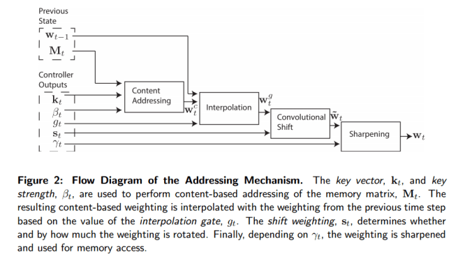
The combined addressing solution works as follows. Firstly the content-addressing weightings are calculated. Then these weightings are blended with those from the previous time-step according to an interpolation gate scalar g ∈ (0,1) emitted by each head to produce the gated weighting.

w_t^g = g_tw_t^c + (1 – g_t)w_t-1

The heads then produce a shift weighting that defines a normalised distribution over the allowed integer shifts (for the location addressing part).

For example, if shifts between -1 and 1 are allowed, s_t has three elements corresponding to the degree to which shifts of -1, 0 and 1 are performed. The simplest way to define the shift weightings is to use a softmax layer of the appropriate size attached to the controller.

The combined process looks like this:

Evaluations

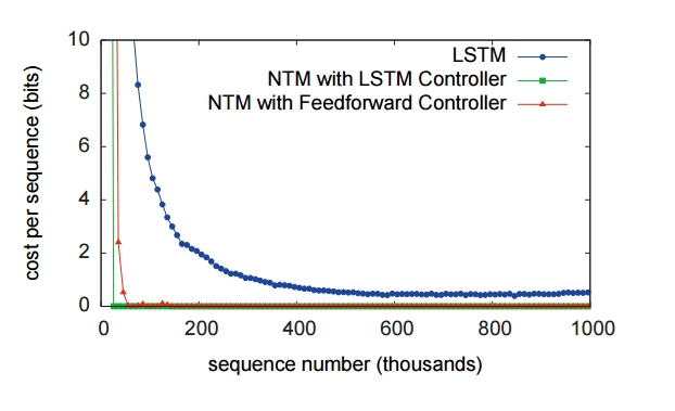
You can see in the following figure that the LSTM based NTM significantly outperforms a standard LSTM on the copy task discussed earlier.

What’s also very interesting is this breakdown of how the NTM actually uses its memory during the copy task (you can see the weightings in the address vector moving along the memory over time).

Similar evaluations are done for a repeating copy task, an associative memory task, an N-gram emulator, and a priority sort! It’s fascinating to see how the machine learns to use its memory and well worth looking into the full paper for.