Universal adversarial perturbations Moosavi-Dezfooli et al., CVPR 2017.
I’m fascinated by the existence of adversarial perturbations – imperceptible changes to the inputs to deep network classifiers that cause them to mis-predict labels. We took a good look at some of the research into adversarial images earlier this year, where we learned that all deep networks with sufficient parameters appear to be vulnerable, and that there are no currently known defences. While that research focused on generating a perturbation that would cause a particular input image to be misclassified, in today’s paper Moosavi-Dezfooli et al., show us how to create a single perturbation that causes the vast majority of input images to be misclassified. Understanding the limits of our models helps us to understand a little more of how they work.
In 20th century warfare, we used camouflage to cause onlookers to mis-predict the label of what they were looking at (“that’s not a tank, it’s just part of the vegetation or whatever.”)
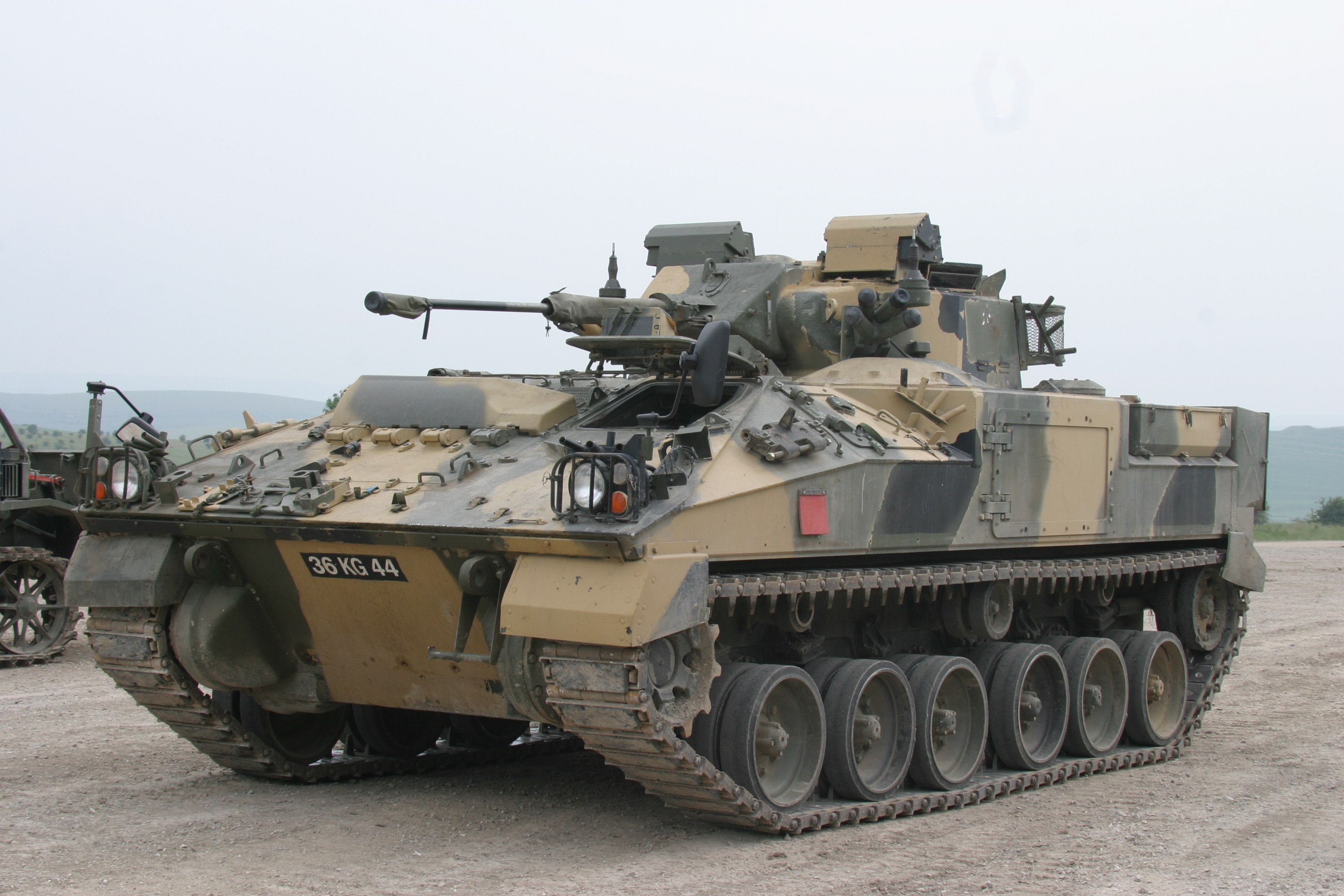
In the 21st century, if we end up in some AI-powered version of warfare (sadly, that seems pretty inevitable at some point), the barely perceptible when applied camouflage pattern used to fool the enemy AI systems is probably going to look something like this:
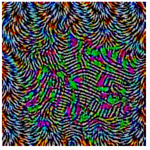
Watch this short video to see it in action. (I’m not quite sure what lead me to such a dark analogy there! Let’s get back to the plot…)
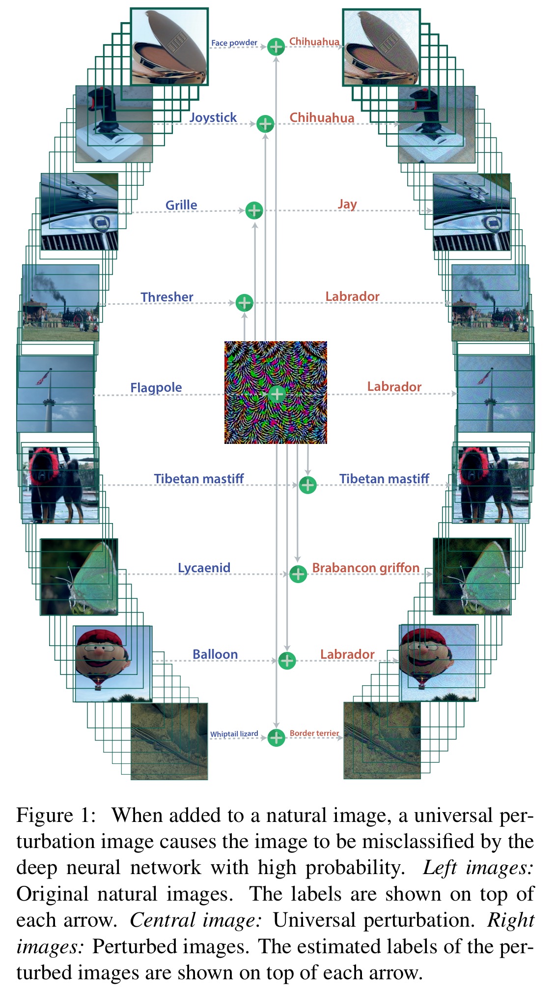
To get an idea of how universal perturbations work, take a look at the following figure which shows correctly classified original input images on the left, and a single perturbation image in the centre which when added to each of the input images causes most of them to be misclassified.
To a human eye, the perturbation is hard to detect. Here are a set of perturbed images – at first glance, other than the unusual labels (showing the mispredictions) you’d be hard pressed to notice anything different. If you zoom in a little closer though, you can make out the swirling pattern. It’s most prominent in, for example, the background sky in the picture of the camel/three-toed sloth.
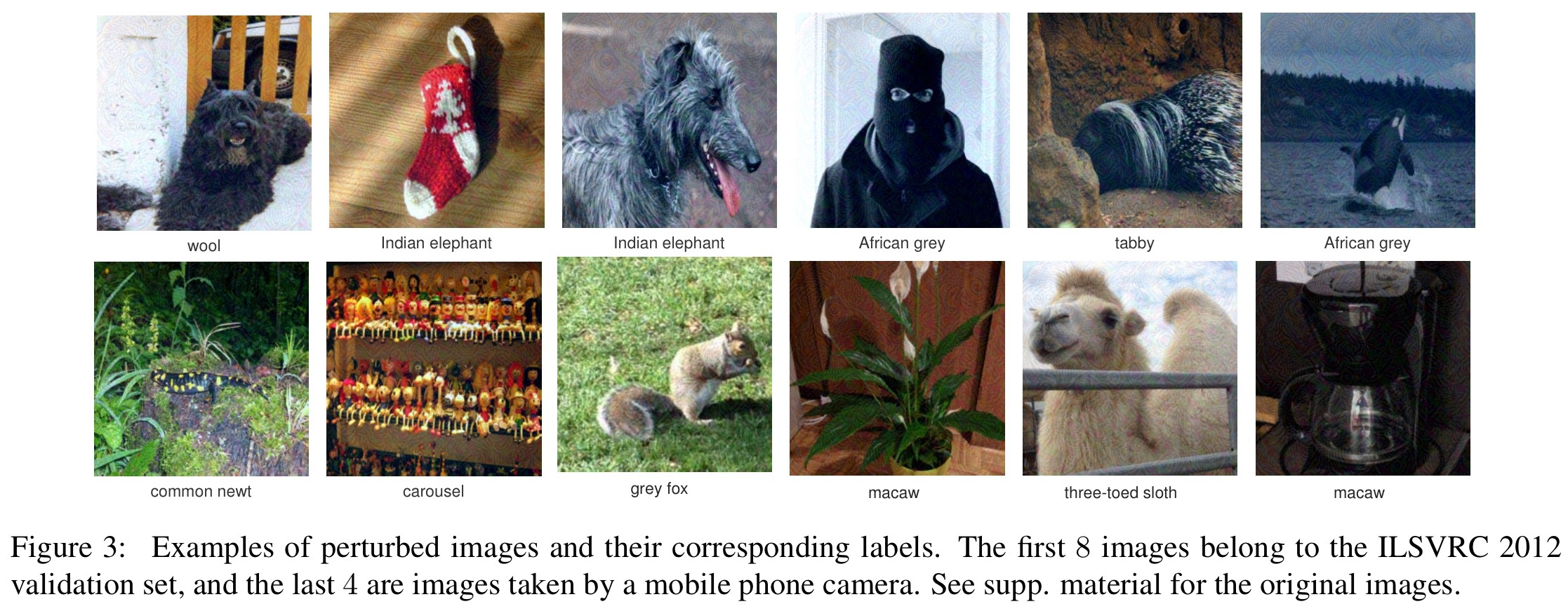
(Enlarge)
How to compute a universal perturbation
For a given (natural image in this paper) classifier, the goal is to find some image (perturbation vector) 


The parameter
controls the magnitude of the perturbation vector
, and
quantifies the desired fooling rate for all images sampled from the distribution.
The perturbation is developed iteratively. In each iteration we sample a data point 

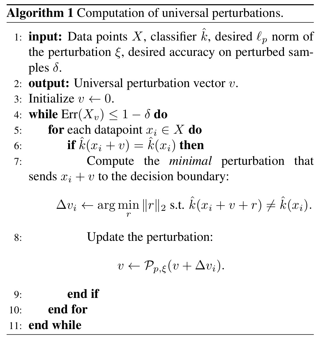
Since the algorithm just finds a random acceptable perturbation image, it can be used to generate multiple universal perturbations for a given deep neural network.
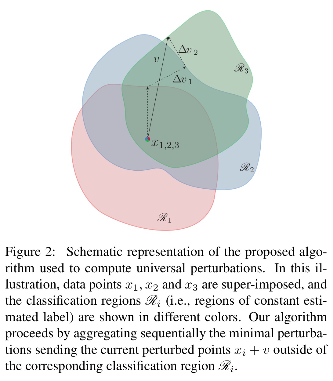
Here’s a picture illustrating how the algorithm proceeds:
Universal perturbations for some common deep networks
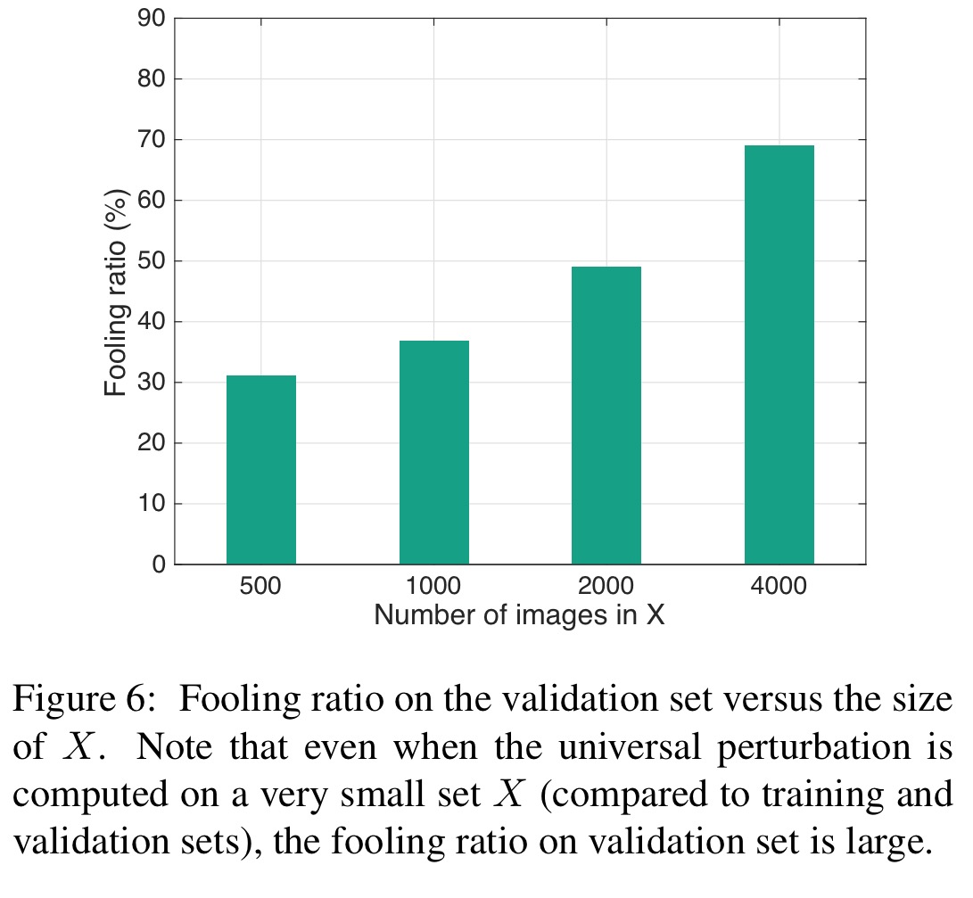
Following the method above, universal perturbations are learned for the ILSVRC 2012 image dataset (training on the set denoted X in the table below), and then those perturbations are tested on a 50,000 image validation set – not used to compute the perturbation – to see how many of them it causes a classifier to fool. The experiment is repeated with for several recent deep neural networks used with ILSVRC 2012.
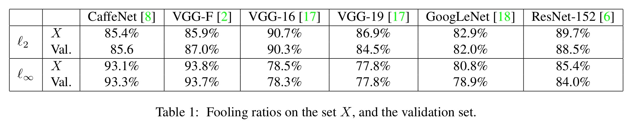
Observe that for all networks, the universal perturbation achieves very high fooling rates on the validation set. Specifically, the universal perturbations computed for CaffeNet and VGG-F fool more than 90% of the validation set.
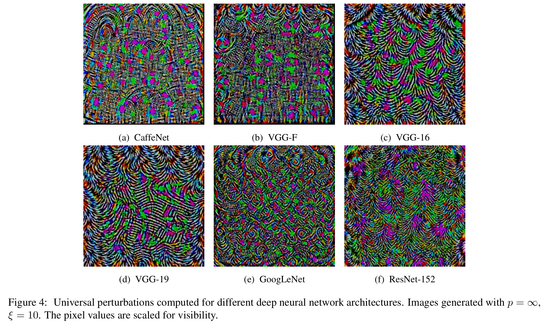
The computed perturbations for the different architectures are shown below.
The universal perturbations computed using Algorithm 1 have … a remarkable generalization power over unseen data points, and can be computed on a very small set of training images.
Do universal perturbations generalise across networks too?
So we’ve seen that universal perturbations can be created for a given model, but does a perturbation developed for one model also fool different models? To a reasonably high degree, yes! The universal perturbations computed for the VGG-19 network, for example, have a fooling ratio above 53% for all other tested architectures.
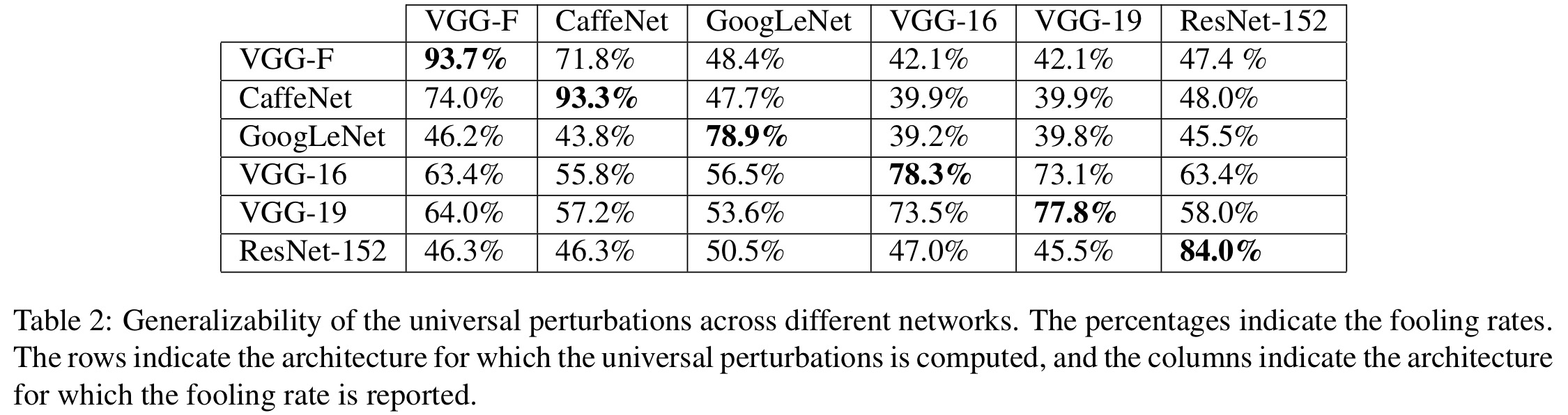
This result shows that such perturbations are of practical relevance, as they generalize well across data points and architectures. In particular, in order to fool a new image on an unknown neural network, a simple addition of a universal perturbation computed on the VGG-19 architecture is likely to misclassify the data point.
Does fine-tuning on perturbations improve resiliency?
If you take the perturbed images that fool a classifier, and fine-tune training using them, you can reduce the fooling rate a bit. After five extra training epochs of VGG-F for example, the misclassification rate drops to 76.2% from 93.7%. However, repeating the process by computing new perturbations and then fine-tuning again seems to yield no further improvements, regardless of the number of iterations, with the fooling ratio hovering around 80%.
Why do universal perturbations work?
If you build a graph where the vertices are labels, and an edge from label i to label j indicates that the majority of images of class i are fooled into label j, then a peculiar topology arises.
In particular, the graph is a union of disjoint components, where all edges in one component mostly connect to one target label.
For example, many image classes are mis-predicted as ‘great grey owl’ or ‘pillow’ in the extracts below.
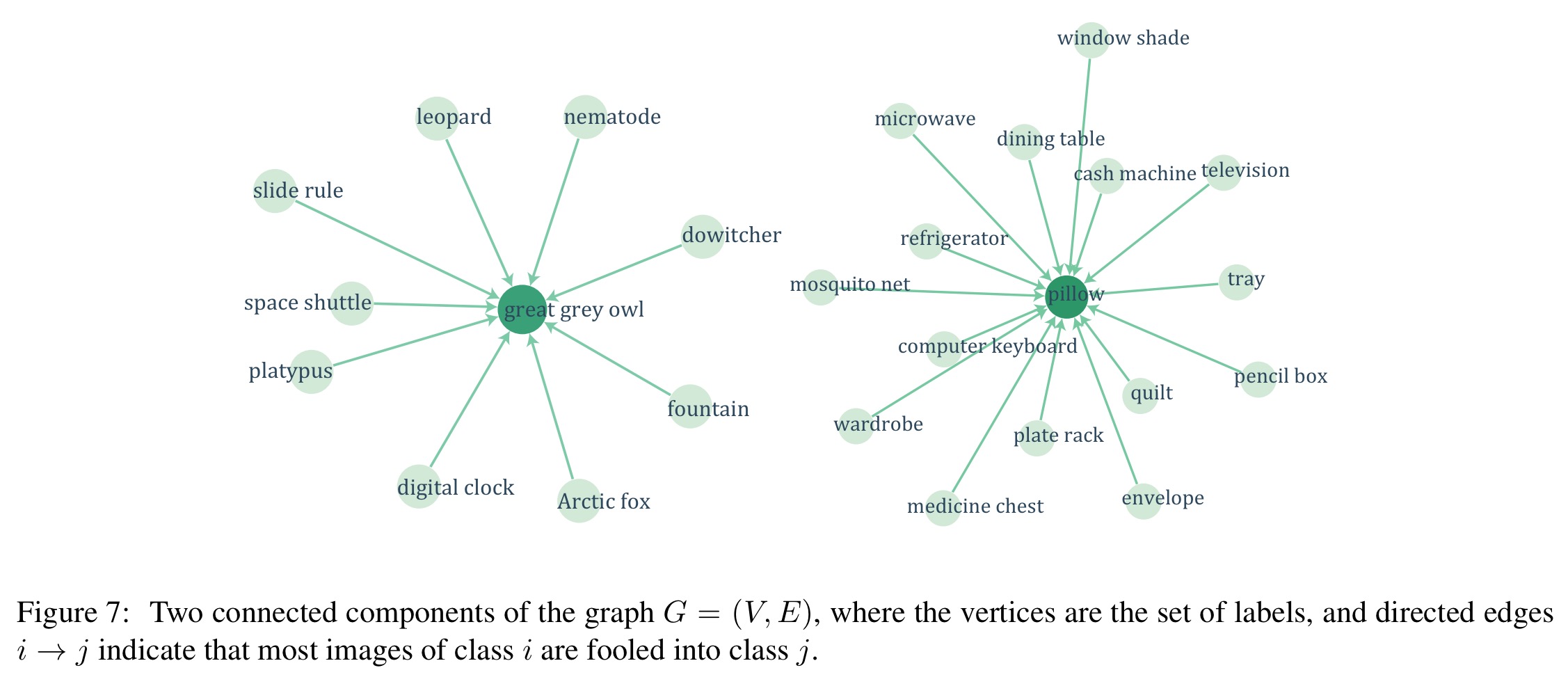
We hypothesize that these dominant labels occupy large regions in the image space, and therefore represent good candidate labels for fooling most natural images.
In another experiment, the authors compare the fooling rates of universal perturbations versus random perturbations and find that universal perturbations are dramatically more effective.
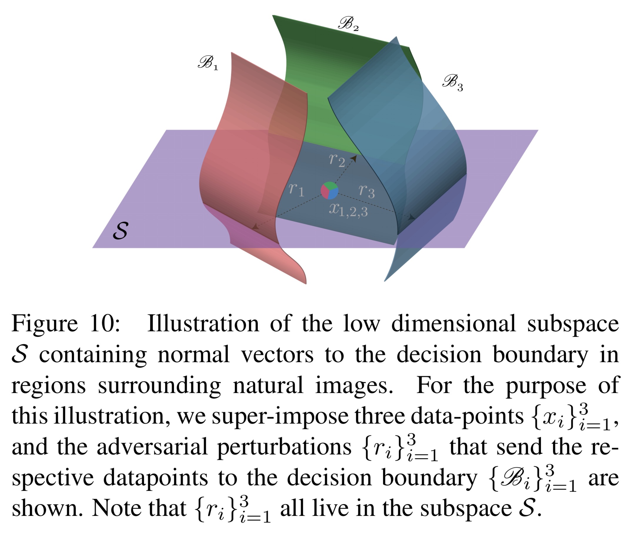
The large difference between universal and random perturbations suggests that the universal perturbation exploits some geometric correlations between different parts of the decision boundary of the classifier.
By exploring vectors that are normal to the decision boundary of the classifier for a given input image, the authors demonstrate the likely existence of a subspace 

Figure 10 (below) illustrates the subspace S that captures the correlations in the decision boundary. It should further be noted that the existence of this low dimensional subspace explains the surprising generalization properties of universal perturbations obtained in Fig. 6, where one can build relatively generalizable universal perturbations with very few images.
A video demonstrating the effect of universal perturbations on a smartphone can be found here.

According to Ian Goodfellow on twitter, this is mostly a rehashing of his ideas from 2015
Some of Goodfellow’s writings on the subject in 2015 are covered here: https://blog.acolyer.org/2017/02/28/when-dnns-go-wrong-adversarial-examples-and-what-we-can-learn-from-them/ , along with a bunch of other related stuff.
He has claimed it without providing any significant evidence, except an ambiguous sentence in the conclusion of one of his works. Scientific method is about providing convincing evidence not throwing random observations.
May be of interest of the readers here
https://arxiv.org/abs/1711.05929
Ooh, thank you! That’s going on my must-read list :)