Yesterday we looked at a series of papers on DNN understanding, generalisation, and transfer learning. One additional way of understanding what’s going on inside a network is to understand what can break it. Adversarial examples are deliberately constructed inputs which cause a network to produce the wrong outputs (e.g., misclassify an input image). We’ll start by looking at ‘Deep Neural Networks are Easily Fooled’ from the ‘top 100 awesome deep learning papers list,’ and then move on to some other examples cited in the excellent recent OpenAI post on “Attacking machine learning with adversarial examples.”
The papers we’ll be covering today are therefore:
- Deep neural networks are easily fooled, Nguyen et al., 2015
- Practical black-box attacks against deep learning systems using adversarial examples, Papernot et al., 2016
- Adversarial examples in the physical world, Goodfellow et al., 2017
- Explaining and harnessing adversarial examples, Goodfellow et al., 2015
- Distillation as a defense to adversarial perturbations against deep neural networks, Papernot et al., 2016
- Vulnerability of deep reinforcement learning to policy induction attacks, Behzadan & Munir, 2017
- Adversarial attacks on neural network policies, Huang et al. 2017
Might I suggest two cups of coffee for this one…
Deep neural networks are easily fooled
What’s this?
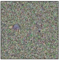
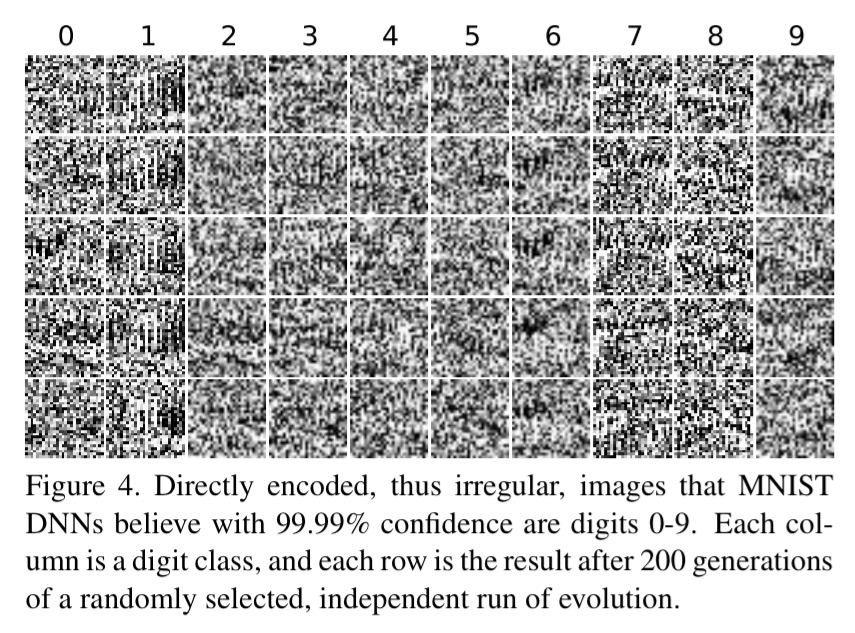
Clearly it’s an armadillo! I’ll make it easier for you… these are five different images of a digit between 0 and 9, but which one?

(It’s a 4, obviously).
What you’re seeing here are adversarial images, deliberately crafted to classify as some class x, while clearly looking nothing like the target class from a human perspective.
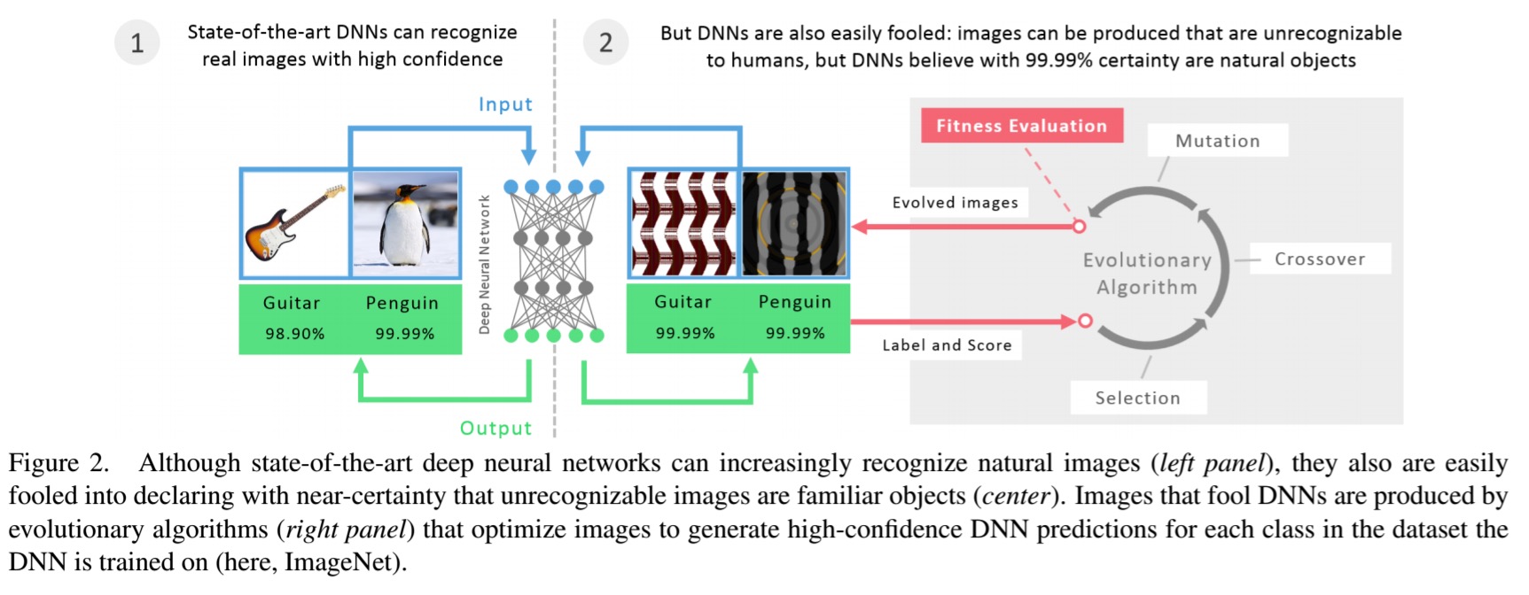
… it is easy to produce images that are completely unrecognizable to humans, but that state-of-the-art DNNs believe to be recognizable objects with 99.99% confidence (e.g., labelling with certainty that white noise static is a lion).
The fact that we can do this tells us something about interesting about the differences between DNN vision and human vision. Clearly, the DNNs are not learning to interpret images in the same way that we do.
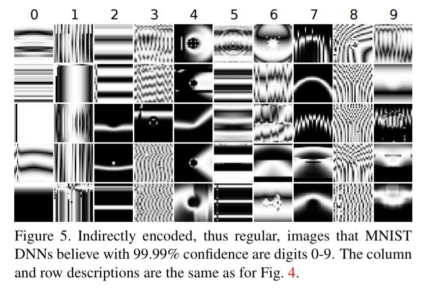
The adversarial images are created using an evolutionary algorithm (EA) that evolves a population of images. Standard EAs use a single fitness function, but the authors here use a new algorithm called MAP-Elites that allows simultaneous evolution of a population containing individuals scoring well on many classes – in each round the best individual so far for each objective is kept. Two different mutation strategies are tested: one that directly encodes pixels in grayscale and then mutates their values, and one that uses an indirect encoding based on a compositional pattern-producing network (CPNN) which can evolve complex regular images that resemble natural and man-made objects.
Take MNIST as an example (digits 0-9). Starting with clean images, within 50 generations images are produces that MNIST DNNs will misclassify with 99.99% confidence but are unrecognisable as such. These images were created used the direct encoding mutation:
And these were created using the indirect encoding mutation:
Using the CPNN encoding and deliberately evolving images to match target DNN classes results in a wide variety of images:
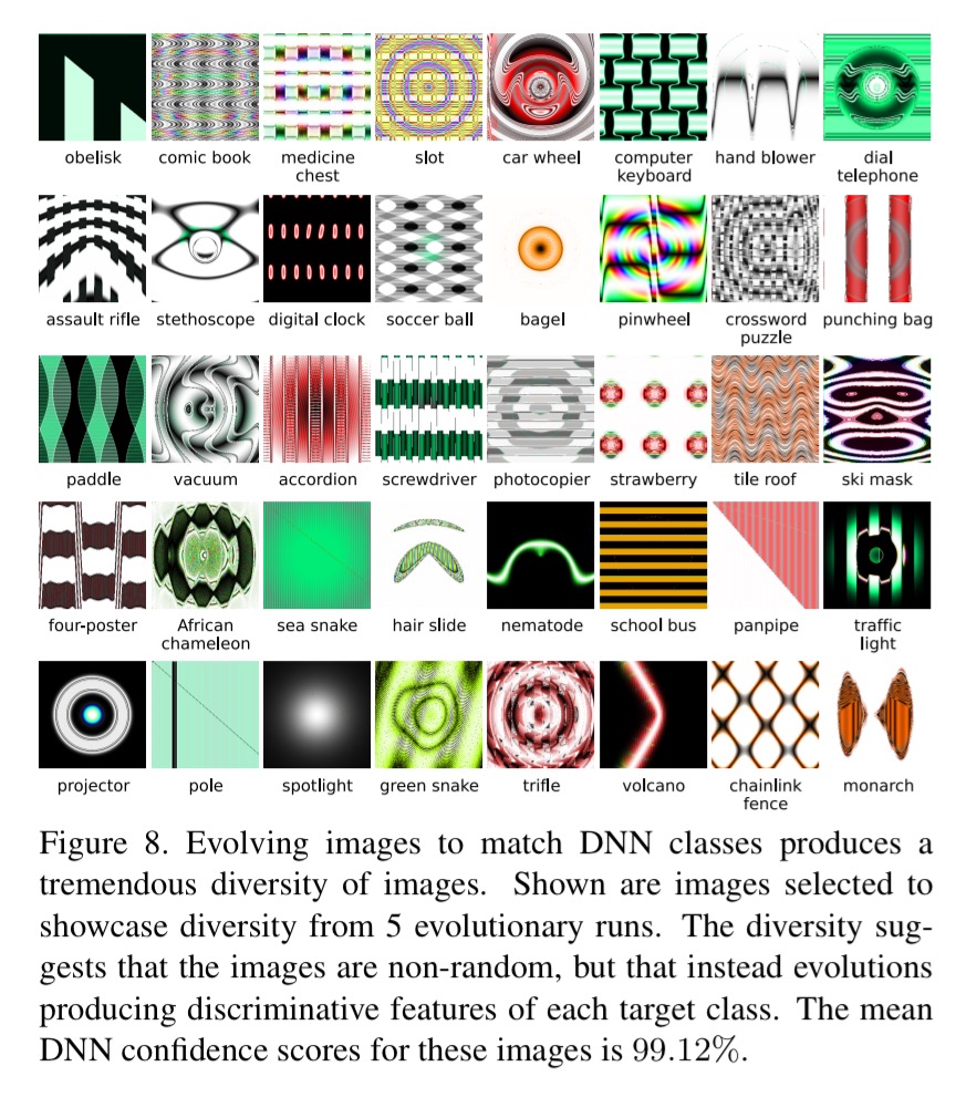
For many of the produced images, one can begin to identify why the DNN believes the image is of that class once given the class label. This is because evolution need only produce features that are unique to, or discriminative for, a class, rather than produce an image that contains all of the typical features of a class.
By removing some of the repeated elements from the generated images, the confidence score of the DNN drops. “These results suggest that DNNs tend to learn low and middle-level features rather than the global structure of objects.”
You might wonder if we can make a DNN more robust to such adversarial images by extending the training regime to include such negative examples. The authors tried this, but found that it was always possible to generate new adversarial examples that still fooled the resulting network (this remained true even after 15 iterations of the process).
Why is it so easy to generate adversarial examples? Discriminative models create decision boundaries that partition data into classification regions. In a high-dimensional input space, the area a model allocates to a class may be much larger than the area occupied by training examples for the class. This leaves plenty of room for adversarial images…
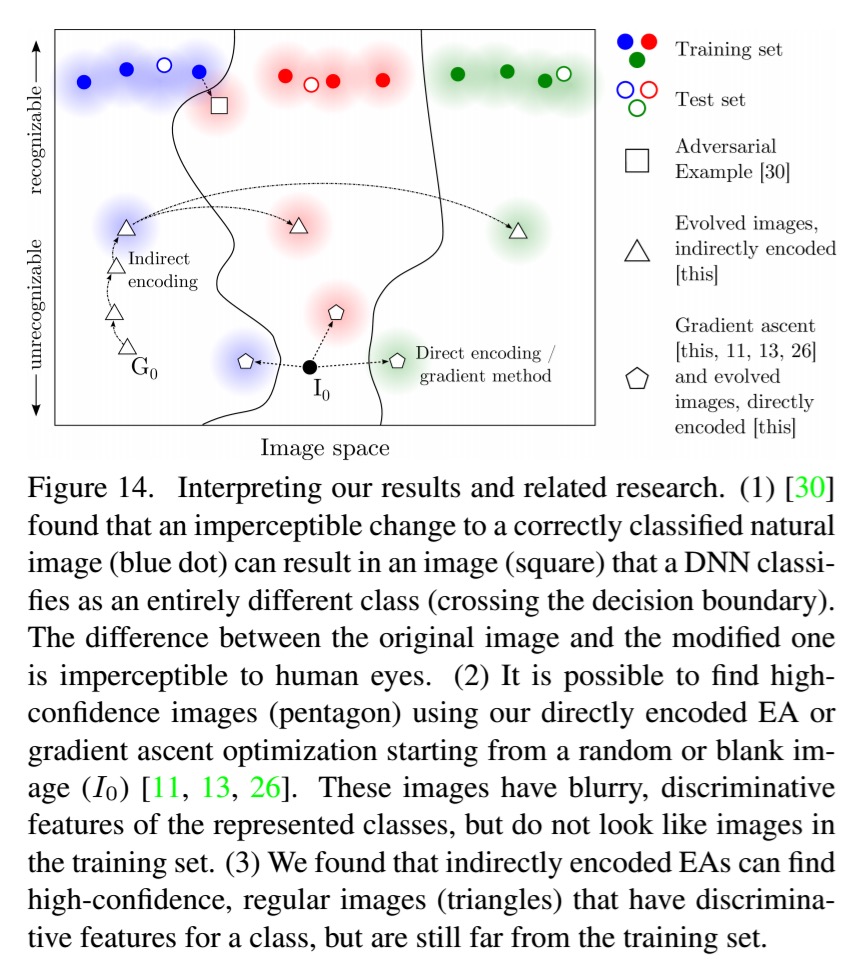
We now turn our attention from adversarial examples as a way of understanding what DNNs are doing, to adversarial examples as a way of attacking DNNs..
The fact that DNNs are increasingly used in a wide variety of industries, including safety-critical ones such as driverless cars, raises the possibility of costly exploits via techniques that generate fooling images…
Practical black-box attacks against deep learning systems using adversarial examples
This is a panda (59.7% confidence):

But this is obviously a gibbon (99.3% confidence):
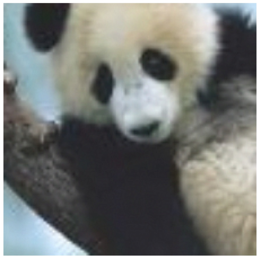
(From ‘Explaining and harnessing adversarial examples,’ which we’ll get to shortly).
The goal of an attacker is to find a small, often imperceptible perturbation to an existing image to force a learned classifier to misclassify it, while the same image is still correctly classified by a human. Previous techniques for generating adversarial images relied on either access to the full training set, and/or the hidden weights in the network. What this paper shows is that successful attacks can be mounted even without such information – all you need is the ability to pass an input to the classifier, and learn the resulting predicted class.
Our threat model thus corresponds to the real-world scenario of users interacting with classifiers hosted remotely by a third-party keeping the model internals secret. In fact, we instantiate our attack against classifiers served by MetaMind, Amazon, and Google. Models are automatically trained by the hosting platform. We are capable of making labeling prediction queries only after training is completed. Thus, we provide the first correctly blinded experiments concerning adversarial examples as a security risk.
The attack works by training a substitute model (owned by the attacker) using the target DNN as an oracle. Target inputs are synthetically generated, passed to the oracle (system under attack), and the output labels becomes the training labels for the substitute model. One the substitute DNN has been trained, adversarial images can be created that succeed against the substitute DNN, using normal white box techniques.
Crucially, the images that fool the substitute network also turn out to often force the same misclassifications in the target model. Since the attacker only needs to (presumably) find one such image that transfers successfully this should be possible with high likelihood. It doesn’t even matter if the substitute DNN has a different architecture to the target model (which it likely will, because we assume the attacker does not know the target architecture) – so long as the substitute DNN is appropriate to the kind of classification task (e.g. CNN for image classification) the attack works well. In fact, the attack doesn’t only work with DNN targets – it generalizes to additional machine learning models (tested with logistic regression, SVMs, decision trees, and nearest neighbours).
The authors showed the ability to attack networks blind by using three cloud ML services provide by MetaMind, Google, and Amazon respectively. In each case training data is uploaded to the service, which learns a classifier (the user has no idea what model the service uses for this). Then the substitute network technique is used to find examples that fool the learned classifier.
An adversary using our attack model can reliably force the DNN trained using MetaMind on MNIST to misclassify 82.84% of adversarial examples crafted with a perturbation not affecting human recognition.
An Amazon classifier that achieved 92.17% test accuracy on MNIST could be fooled by 96.19% of adversarial examples. The Google classifier achieved 92% test accuracy on MNIST and could be fooled by 88.94% of adversarial examples. Defences based on gradient masking are not effective against the substitute attack.
Adversarial examples in the physical world
So now we know that you don’t need access to a model in order to successfully attack it. But there’s more…
Up to now, all previous work has assumed a threat model in which the adversary can feed data directly into the machine learning classifier. This is not always the case for systems operating in the physical world, for example those which are using signals from cameras and other sensors as input. This paper shows that even in such physical world scenarios, machine learning systems are vulnerable to adversarial examples. We demonstrate this by feeding adversarial images obtained from a cell-phone camera to an ImageNet Inception classifier and measuring the classification accuracy of the system. We find that a large fraction of adversarial examples are classified incorrectly even when perceived through the camera.
The authors print clean and adversarial images, take photos of the printed images, crop those photos to be the same size as the originals, and then pass these into the classifier. The procedure takes place with manual photography and no careful control of lighting, camera angle etc., thus in introduces nuisance variability with the potential to destroy adversarial perturbations depending on subtle changes.
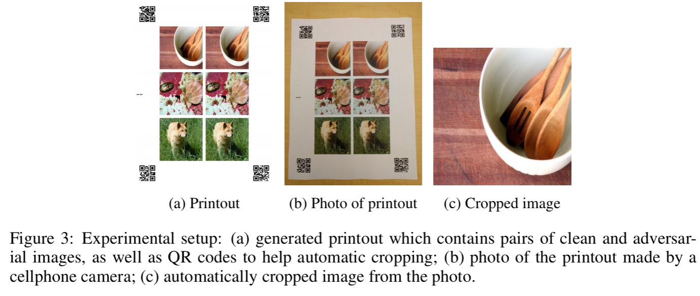
Overall, the results show that some fraction of adversarial examples stays misclassified even after a non-trivial transformation: the photo transformation. This demonstrates the possibility of physical adversarial examples. For example, an adversary using the fast method with ε = 16 could expect that about 2/3 of the images would be top-1 misclassified and about 1/3 of the images would be top-5 misclassified. Thus by generating enough adversarial images, the adversary could expect to cause far more misclassification than would occur on natural inputs.
Other physical attacks mentioned in prior work include generation of audio inputs that mobile phones recognise as intelligible voice commands but humans hear as an unintelligible voice, and face recognition systems fooled by previously captured images of an authorized user’s face…
An adversarial example for the face recognition domain might consist of very subtle markings applied to a person’s face, so that a human observer would recognize their identity correctly, but a machine learning system would recognize them as being a different person.
Explaining and harnessing adversarial examples
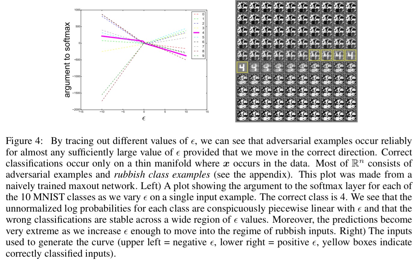
Why do these adversarial examples work? Goodfellow et al. show us that all we need in order to be vulnerable is linear behavior in a high-dimensional space.
[The] results suggest that classifiers based on modern machine learning techniques, even those that obtain excellent performance on the test set, are not learning the true underlying concepts that determine the correct output label. Instead, these algorithms have built a Potemkin village that works well on naturally occuring data, but is exposed as a fake when one visits points in space that do not have high probability in the data distribution.
Consider a high-dimensional linear classifier, where the weight vector w has n dimensions. Each individual input feature has limited precision (e.g., using 8 bits per pixel in digital images, thus discarding all information below 1/255 of the dynamic range). For any one input, making a small change (smaller than the precision of the features) would not be expected to change the overall prediction of the classifier. However…
… we can make many infinitesimal changes to the input that add up to one large change to the output. We can think of this as a sort of ‘accidental steganography,’ where a linear model is forced to attend exclusively to the signal that aligns most closely with its weights, even if multiple signals are present and other signals have much greater amplitude.
We can maximise the impact of the many small changes by aligning the changes with the sign of the corresponding weight. This turns out to be a fast way of generating adversarial images.
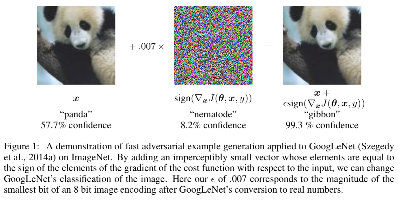
An intriguing aspect of adversarial examples is that an example generated for one model is often misclassified by other models, even when they have different architecures or were trained on disjoint training sets. Moreover, when these different models misclassify an adversarial example, they often agree with each other on its class. Explanations based on extreme non-linearity and overfitting cannot readily account for this behavior…
But under the linear explanation, adversarial examples occur in broad subspaces – this explains why adversarial examples are abundant and why an example misclassified by one classifier has a fairly high probability of being misclassified by another. It’s the direction of perturbation, rather than the specific point in space, that matters most.
Our explanation suggests a fundamental tension between designing models that are easy to train due to their linearity and designing models that use nonlinear effects to resist adversarial perturbation. In the long run, it may be possible to escape this tradeoff by designing more powerful optimization methods that can successfully train more nonlinear models.
Distillation as a defense to adversarial perturbations against deep neural networks
Yesterday we looked at distillation as a way of transferring knowledge from large models to smaller models. In ‘Distillation as a defense…,’ Papernot et al. show that the distillation technique (training using the probability distribution as the target, not just the argmax class label) can also be used to greatly reduce the vulnerability of networks to adversarial perturbations.
We formulate a new variant of distillation to provide for defense training: instead of transferring knowledge between different architectures, we propose to use the knowledge extracted from a DNN to improve its own resilience to adversarial samples.
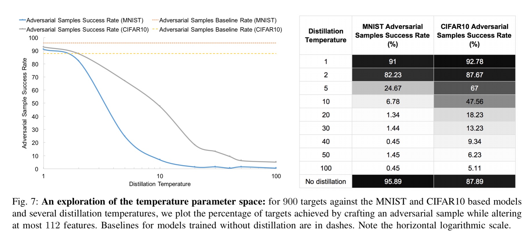
With a DNN trained on the MNIST dataset, defensive distillation reduces the success rate of adversarial sample crafting from 95.89% to just 0.45%! For a DNN trained on the CIFAR dataset, the success rate was reduced from 87.89% to 5.11%. In fact, defensive distillation can reduce the sensitivity of a DNN to input perturbations by a whopping factor of 1030. This increases the minimum number of input features that need to be perturbed for adversarial samples to succeed by up to 8x in tests.
Here are some examples from MNIST and CIFAR showing legitimate and adversarial samples:
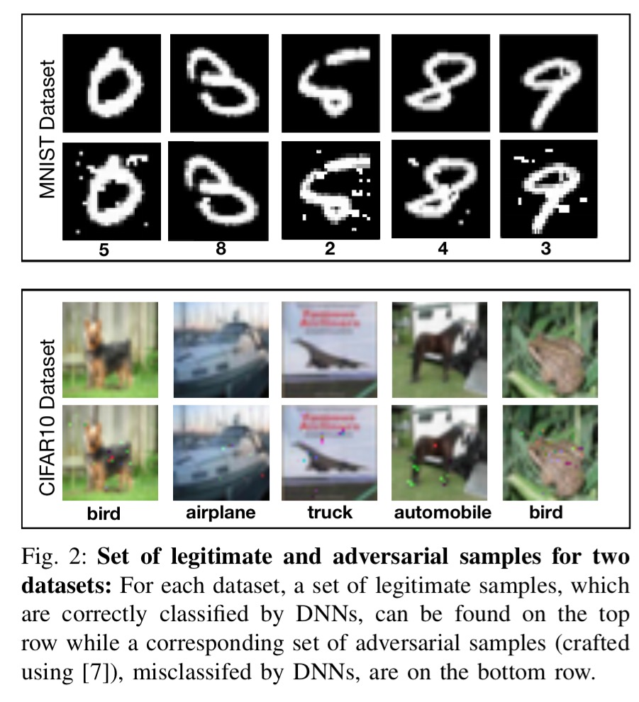
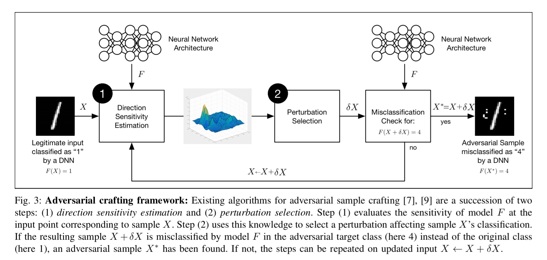
So how and why does defensive distillation work? Consider a general adversarial crafting framework that works by first figuring out the directions around a given input sample in which the model learned by a DNN is most sensitive, and then uses this information to select a perturbation among the input dimensions.
If the direction gradients are steep, we can make a big impact with small perturbations, but if they are shallow this is much harder to achieve. Think about the difference between being on a ‘ridge’ in the classification space whereby a small move to either side could see you tumbling down the mountain, and being on a plateau where you can freely wander around without much consequence.
To defend against such perturbations, one must therefore reduce these variations around the input, and consequently the amplitude of adversarial gradients. In other words, we must smooth the model learned during training by helping the network generalize better to samples outside of its training dataset.
The ‘robustness’ of a DNN to adversarial samples is correlated with classifying inputs relatively consistently in the neighbourhood of a given sample.
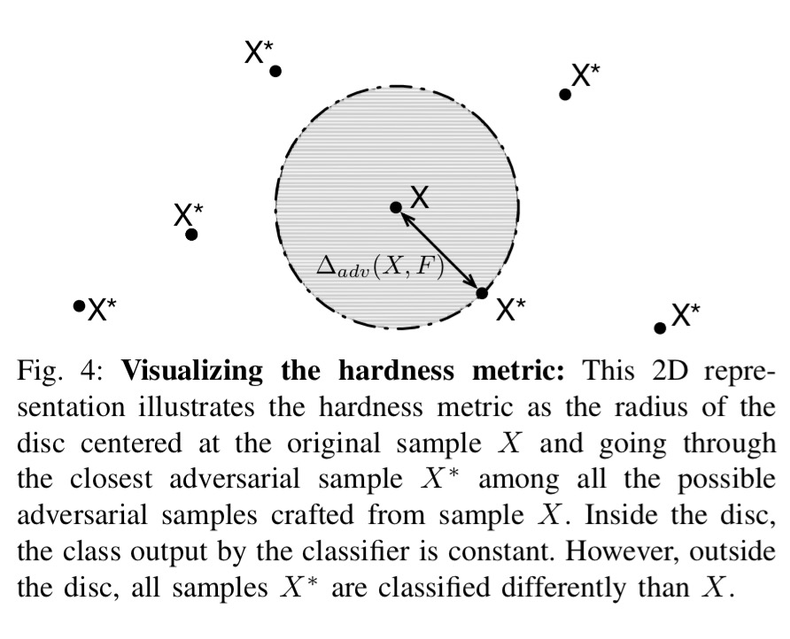
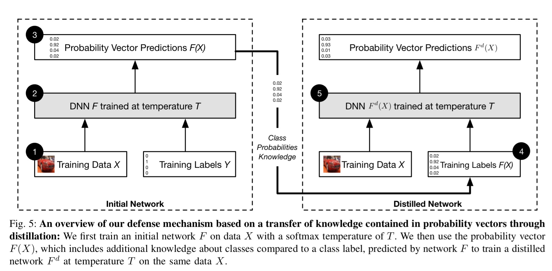
To achieve this smoothing, distillation defense first trains a classification network as normal. Then we take another fresh model instance with the exact same architecture (no need to transfer to a smaller model) and train it using the probability vectors learned by the first model.
The main difference between defensive distillation and the original distillation proposed by Hinton et al. is that we keep the same network architecture to train both the original network as well as the distilled network. This difference is justified by our end which is resilience instead of compression.
Training the network in this way with explicit relative information about classes prevents it from fitting too tightly to the data, and hence contributes to better generalization.
The following figure shows how the distillation temperature impacts the model’s ability to defend against adversarial samples. Intuitively, the higher the temperature the greater the smoothing, and thus the better the defence.
Distillation has only a small impact on classification accuracy, and may even improve it!
We know that many different machine learning models are vulnerable to adversarial attacks, but the defensive distillation defense is only applicable to DNN models that produce an energy-based probability distribution for which a temperature can be defined…
However, note that many machine learning models, unlike DNNs, don’t have the model capacity to be able to resist adversarial examples… A defense specialized to DNNs, guaranteed by the universal approximation property to at least be able to represent a function that correctly processes adversarial examples, is thus a significant step towards building machine learning models robust to adversarial samples.
This all sounds quite promising… unfortunately a subsequent paper showed that even defensive distillation is insufficient in mitigating adversarial examples :(, ‘Defensive distillation is not robust to adversarial examples.’
In this short paper, we demonstrate that defensive distillation is not effective. We show that, with a slight modification to a standard attack, one can find adversarial examples on defensively distilled networks. We demonstrate the attack on the MNIST digit recognition task. Distillation prevents existing techniques from finding adversarial examples by increasing the magnitude of the inputs to the softmax layer. This makes an unmodified attack fail. We show that if we artificially reduce the magnitude of the input to the softmax function, and make two other minor changes, the attack succeeds. Our attack achieves successful targeted misclassification on 96.4% of images by changing on average 4.7% of pixels.
Damn!
Vulnerability of deep reinforcement learning to policy induction attacks
If you weren’t there already, this is where we get to the ‘Oh *#@!’ moment! We’ve seen that classifiers can be fooled, but this paper and the next one show us that deep reinforcement learning networks (e.g. DQNs) are also vulnerable to adversarial attack. The attack is demonstrated on Atari games (what else!), but the broader implications are sobering:
The reliance of RL on interactions with the environment gives rise to an inherent vulnerability which makes the process of learning susceptible to perturbation as a result of changes in the observable environment. Exploiting this vulnerability provides adversaries with the means to disrupt or change control policies, leading to unintended and potentially harmful actions. For instance, manipulation of the obstacle avoidance and navigation policies learned by autonomous Unmanned Aerial Vehicles (UAV) enables the adversary to use such systems as kinetic weapons by inducing actions that lead to intentional collisions.
Fortunately, we’ve already seen many of the building blocks needed to craft the attack, so we can describe it quite succinctly. The goal of the attacker is to fool a DQN into taking an action (inducing an arbitrary policy) chosen by the attacker. The assumed threat model is similar to the ‘black-box’ model we saw earlier in this post: the attacker has no visibility of the insides of the DQN, and does not know its reward function. However, the attacker can see the same environmental inputs that the target DQN sees, and it can observe the actions taken by the DQN and hence estimate the reward function.
The first step is to us the ‘Practical black-box attack…’ technique to train a substitute DQN that matches the policies chosen by the target. Following the black-box playbook we now craft adversarial inputs (instead of images) that trigger an incorrect choice of optimal action…
If the attacker is capable of crafting adversarial inputs s’t and s’t+1 such that the value of [the training function] is minimized for a specific action a’, then the policy learned by the DQN at this time-step is optimized for suggesting a’ as the optimal action given the state st.
(An example of adversarial inputs might be manipulating some of the screen input pixels in an Atari game).
At this point we have a DQN which has learned an adversarial policy. The next step in the playbook is to find a way to transfer this learned adversarial policy to the target network. This is done in an exploitation cycle:
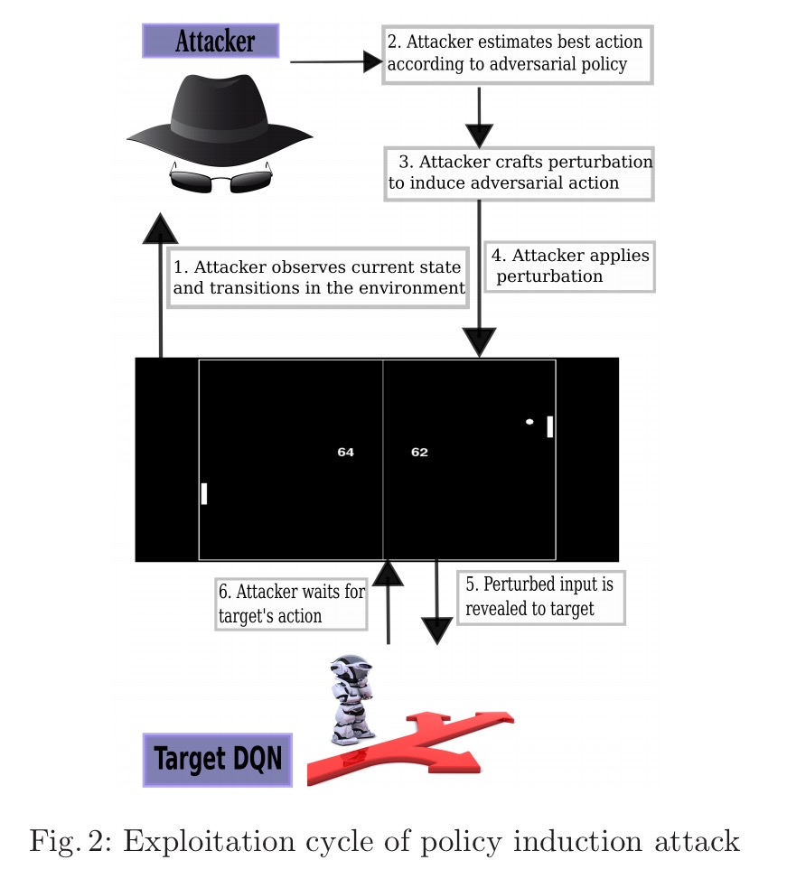
The first question we need to answer therefore, is ‘is it possible to generate adversarial examples for DQNs?’ Fig. 4 below shows that yes, this is indeed possible (game of Atari Pong, using both the Fast Gradient Sign and Jacobian Saliency Map Algorithm approaches to generate adversarial perturbations)
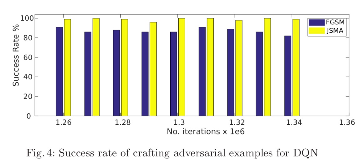
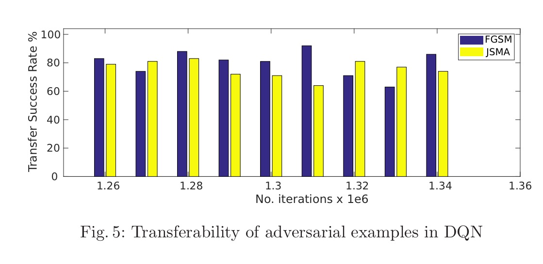
The next question we have to answer, is whether or not these adversarial examples can be transferred. The answer again is yes, with high success rate:
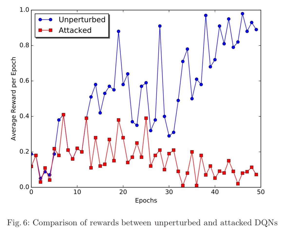
Our final experiment tests the performance of our proposed exploitation mechanism. In this experiment, we consider an adversary whose reward value is the exact opposite of the game score, meaning that it aims to devise a policy that maximizes the number of lost games. To obtain this policy, we trained an adversarial DQN on the game, whose reward value was the negative of the value obtained from target DQN’s reward function…
A picture is worth a thousand words here:
Since all known counter-measures have been shown not to be sufficient,
… it is hence concluded that the current state of the art in countering adverse examples and their exploitation is incapable of providing a concrete defense against such exploitations.
Adversarial attacks on neural network policies
Almost in parallel to the previous paper, Huang et al. published this work which also shows that reinforcement learning networks are vulnerable to adversarial attacks. They demonstrate this across four different Atari games (Chopper Command, Pong, Seaquest, and Space Invaders) using white-box attacks. They also show that the attacks succeed across a range of deep reinforcement learning algorithms (DQN, TRPO, and A3C). Policies trained with TRPO and A3C are more resistant, but not safe from the attack.
Then the authors demonstrate transfer capabilities using black-box attacks too:
We observe that the cross-dataset transferability property also holds in reinforcement learning applications, in the sense that an adversarial example designed to interfere with the operation of one policy interferes with the operation of another policy, so long as both policies have been trained to solve the same task. Specifically, we observe that adversarial examples transfer between models trained using different trajectory rollouts and between models trained with different training algorithms.
Combine this with the lessons we learned above in ‘Adversarial examples in the physical world,’ and as the authors point out, things could get very interesting indeed!
Our experiments show it is fairly easy to confuse such policies with computationally-efficient adversarial examples, even in black-box scenarios. Based on ‘Adversarial examples in the physical world’, it is possible that these adversarial perturbations could be applied to objects in the real world, for example adding strategically-placed paint to the surface of a road to confuse an autonomous car’s lane-following policy

Interesting read.. It might be completely off track but an idea came to mind while reading this. Currently, image recognition networks are bottom-up in the sense that they extract simple features and build upon them using max-pooling layers. What if we built a network in a reverse fashion where coarse and large features are extracted first and refined along the way. (It would probably pose problems with learning and gradient updates though.)
Does this adversarial problem also occurs in traditional image classification like SVM? We could put the hypothesis that one against-all classifier are more robust to this effect. Then we could build an ensemble of binary classifier instead of a single multiclass DNN.
Yes, it can be used against other classifiers: https://youtu.be/hUukErt3-7w?t=9m45s
Great read!
@Michel Lemay interesting idea. I wonder if NNs with multiple inputs could do it – e.g. 1) regular image, plus 2) thumbnail image or coarse / large features extracted during pre-processing. You just have to make sure that the lower layers can calculate high level features, without losing the data required to develop lower level features. –> Perhaps if you just feed in the high-level stuff it would help.
The Space of Transferable Adversarial Examples came out today https://arxiv.org/abs/1704.03453 by Tramèr et al. (Goodfellow is coauthor). Very neat illustrations!