Learning to learn by gradient descent by gradient descent Andrychowicz et al. NIPS 2016

One of the things that strikes me when I read these NIPS papers is just how short some of them are – between the introduction and the evaluation sections you might find only one or two pages! A general form is to start out with a basic mathematical model of the problem domain, expressed in terms of functions. Selected functions are then learned, by reaching into the machine learning toolbox and combining existing building blocks in potentially novel ways. When looked at this way, we could really call machine learning ‘function learning‘.

Thinking in terms of functions like this is a bridge back to the familiar (for me at least). We have function composition. For example, given a function mapping images to feature representations, and a function acting as a classifier mapping image feature representations to objects, we can build a systems that classifies objects in images with .

Each function in the system model could be learned or just implemented directly with some algorithm. For example, feature mappings (or encodings) were traditionally implemented by hand, but increasingly are learned…

The move from hand-designed features to learned features in machine learning has been wildly successful.

Part of the art seems to be to define the overall model in such a way that no individual function needs to do too much (avoiding too big a gap between the inputs and the target output) so that learning becomes more efficient / tractable, and we can take advantage of different techniques for each function as appropriate. In the above example, we composed one learned function for creating good representations, and another function for identifying objects from those representations.

We can have higher-order functions that combine existing (learned or otherwise) functions, and of course that means we can also use combinators.

And what do we find when we look at the components of a ‘function learner’ (machine learning system)? More functions!

Frequently, tasks in machine learning can be expressed as the problem of optimising an objective function defined over some domain .

The optimizer function maps from to . The standard approach is to use some form of gradient descent (e.g., SGD – stochastic gradient descent). A classic paper in optimisation is ‘No Free Lunch Theorems for Optimization’ which tells us that no general-purpose optimisation algorithm can dominate all others. So to get the best performance, we need to match our optimisation technique to the characteristics of the problem at hand:

… specialisation to a subclass of problems is in fact the only way that improved performance can be achieved in general.

Thus there has been a lot of research in defining update rules tailored to different classes of problems – within deep learning these include for example momentum, Rprop, Adagrad, RMSprop, and ADAM.

But what if instead of hand designing an optimising algorithm (function) we learn it instead? That way, by training on the class of problems we’re interested in solving, we can learn an optimum optimiser for the class!

The goal of this work is to develop a procedure for constructing a learning algorithm which performs well on a particular class of optimisation problems. Casting algorithm design as a learning problem allows us to specify the class of problems we are interested in through example problem instances. This is in contrast to the ordinary approach of characterising properties of interesting problems analytically and using these analytical insights to design learning algorithms by hand.

If learned representations end up performing better than hand-designed ones, can learned optimisers end up performing better than hand-designed ones too? The answer turns out to be yes!

Our experiments have confirmed that learned neural optimizers compare favorably against state-of-the-art optimization methods used in deep learning.

In fact not only do these learned optimisers perform very well, but they also provide an interesting way to transfer learning across problems sets. Traditionally transfer learning is a hard problem studied in its own right. But in this context, because we’re learning how to learn, straightforward generalization (the key property of ML that lets us learn on a training set and then perform well on previously unseen examples) provides for transfer learning!!

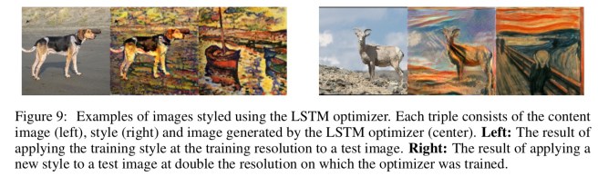
We witnessed a remarkable degree of transfer, with for example the LSTM optimizer trained on 12,288 parameter neural art tasks being able to generalize to tasks with 49,512 parameters, different styles, and different content images all at the same time. We observed similar impressive results when transferring to different architectures in the MNIST task.

Learning how to learn

Thinking functionally, here’s my mental model of what’s going on… In the beginning, you might have hand-coded a classifier function, , which maps from some Input to a Class:

    c :: Input -> Class

With machine learning, we figured out for certain types of functions it’s better to learn an implementation than try and code it by hand. An optimisation function takes some TrainingData and an existing classifier function, and returns an updated classifier function:

    type Classifier = (Input -> Class)
    f :: TrainingData -> Classifier -> Classifier

What we’re doing now is saying, “well, if we can learn a function, why don’t we learn f itself?”

    type Optimiser = (TrainingData -> Classifier -> Classifier)
    g :: TrainingData -> Optimiser -> Optimiser

Let be the (to be learned) update rule for our (optimiser) optimiser. We need to evaluate how effective is over a number of iterations, and for this reason is modelled using a recurrent neural network (LSTM). The state of this network at time is represented by .

Suppose we are training to optimise an optimisation function . Let result in a learned set of parameters for , $\theta^*$ The loss function for training uses as _its_ expected loss the expected loss of as trained by .

We can minimise the value of using gradient descent on .

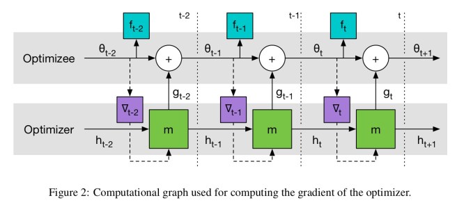
To scale to tens of thousands of parameters or more, the optimiser network m operators coordinatewise on the parameters of the objective function, similar to update rules like RMSProp and ADAM. The update rule for each coordinate is implemented using a 2-layer LSTM network using a forget-gate architecture.

The network takes as input the optimizee gradient for a single coordinate as well as the previous hidden state and outputs the update for the corresponding optimise parameter. We refer to this architecture as an LSTM optimiser.

Learned learners in action

We compare our trained optimizers with standard optimisers used in Deep Learning: SGD, RMSprop, ADAM, and Nesterov’s accelerated gradient (NAG). For each of these optimizers and each problem we tuned the learning rate, and report results with the rate that gives the best final error for each problem.

Optimisers were trained for 10-dimensional quadratic functions, for optimising a small neural network on MNIST, and on the CIFAR-10 dataset, and on learning optimisers for neural art (see e.g. Texture Networks).

Here’s a closer look at the performance of the trained LSTM optimiser on the Neural Art task vs standard optimisers:

And because they’re pretty… here are some images styled by the LSTM optimiser!

A system model and learned components

So there you have it. It seems that in the not-too-distant future, the state-of-the-art will involve the use of learned optimisers, just as it involves the use of learned feature representations today. This appears to be another crossover point where machines can design algorithms that outperform those of the best human designers. And of course, there’s something especially potent about learning learning algorithms, because better learning algorithms accelerate learning…

In this paper, the authors explored how to build a function g to optimise an function f, such that we can write:

where d is some training data.

When expressed this way, it also begs the obvious question what if I write:

or go one step further using the Y-combinator to find a fixed point:

Food for thought…