Unsupervised learning of 3D structure from images
Unsupervised learning of 3D structure from images Rezende et al. (Google DeepMind) NIPS,2016
Earlier this week we looked at how deep nets can learn intuitive physics given an input of objects and the relations between them. If only there was some way to look at a 2D scene (e.g., an image from a camera) and build a 3D model of the objects in it and their relationships… Today’s paper choice is a big step in that direction, learning the 3D structure of objects from 2D observations.
The 2D projection of a scene is a complex function of the attributes and positions of the camera, lights and objects that make up the scene. If endowed with 3D understanding agents can abstract away from this complexity to form stable disentangled representations, e.g., recognizing that a chair is a chair whether seen from above or from the side, under different lighting conditions, or under partial occlusion. Moreover, such representations would allow agents to determine downstream properties of these elements more easily and with less training, e.g., enabling intuitive physical reasoning…
The approach described is this paper uses an unsupervised deep learning end-to-end model and “demonstrates for the first time the feasibility of learning to infer 3D representations of the world in a purely unsupervised manner.”
The overall framework looks like this:
")
An inference network encodes the observed data into a latent 3D representation, 
To capture the complex distribution of 3D structures, we apply recent work on sequential generative models by extending them to operation on different 3D representations. This family of models generates the observed data over the course of T computational steps. More precisely, these models operate by sequentially transforming independently generate Guassian latent variables into refinements of a hidden representation
, which we refer to as the ‘canvas’.
The whole process is succinctly described by a set of six equations:
- The initial values for the hidden latent variables are drawn from a Gaussian distribution:
- The initial context encoding is a function of the context
(something that conditions all instances of inference and generation – in the experiments it is either nothing; an object class label; or one or more views of the scene from different cameras), and the state
at the previous time step:
The particular encoding function used varied by experiment.
- A fully-connected LSTM is used as the transition function
) to update the hidden state.
- The 3D projection
is created as a function of the hidden state:
. The 3D representation can be volumetric or a mesh. When using a volumetric latent 3D representation, the projection equation is parameterized by a volumetric spatial transformer (VST) – details are provided in the appendix.
- The 2D projection
is a projection operator from the model’s latent 3D representation
to the training data’s domain (either a volume or an image in the experiments):
. In the experiments three different kinds of projection operators are used:

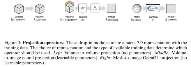
- If the training data is already in the form of volumes (e.g., in medical imagery) then the projection is simply the identity function :
.
- When only access to images captured by a camera is available, then a map from the F-dimensional volume
- When working with a mesh representation, an off-the-shelf OpenGL renderer is used. The renderer is treated as a black box with no parameters.
- Finally, the observation
is simply

How well does it work?
We demonstrate the ability of our model to learn and exploit 3D scene representations in five challenging tasks. These tasks establish it as a powerful, robust and scalable model that is able to provide high quality generations of 3D scenes, can robustly be used as a tool for 3D scene completion, can be adapted to provided class-specific or view-specific generations that allow variations in scenes to be explored, can synthesize multiple 2D scenes to form a coherent understanding of a scene, and can operate with complex visual systems such as graphics renderers.
That’s quite the list! All experiments used LTSMs with 300 hidden neurons and 10 latent variables per generation step.
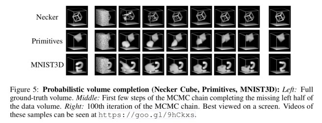
Here’s an example of the model being used to impute missing data in 3D volumes. “This is a capability that is often need to remedy sensor defects that result in missing or corrupt regions.”
And here’s an example where models were trained with a context representing the class of object, and then asked to generate a representative sample:
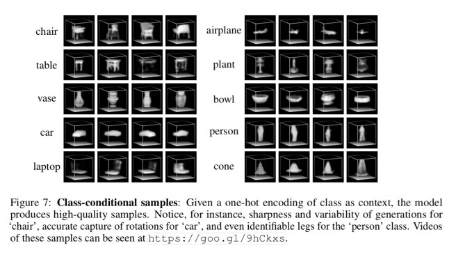
The model produces high-quality samples of all classes. We note their sharpness, and that they accurately capture object rotations, and also provide a variety of plausible generations.
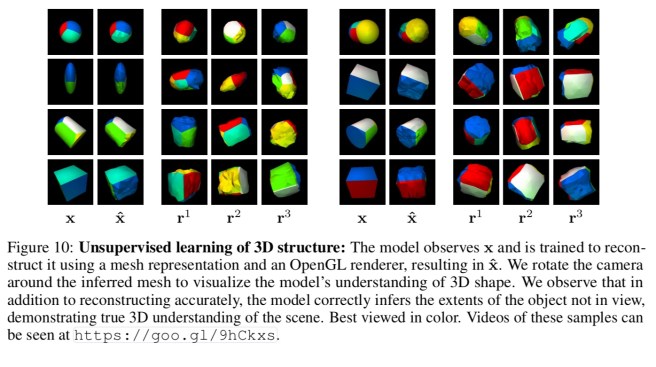
Using a 3D mesh-based representation and training with a fully-fledged black-box renderer in the loop enables learning of the interactions between an objects’ colours, materials and textures, positions of lights, and of other objects. Using a ‘geometric primitives’ dataset with 2D images textured with a colour on each side the model infers the parameters of a 3D mesh and its orientation relative to the camera. When rendered, this 3D mesh accurately reconstructs the original image.

Did someone just crack the holy grail of 2d -> 3d vision. This is amazing. I have always wondered how one can represent an scene graph of containers, nodes, lights and camera in a neural network.
Reblogged this on josephdung.