GraphLab: A new framework for parallel machine learning – Low et al. 2010
In this paper we propose GraphLab, a new parallel framework for ML which exploits the sparse structure and common computational patterns of ML algorithms. GraphLab enables ML experts to easily design and implement efficient scalable parallel algorithms by composing problem specific computation, data-dependencies, and scheduling.
GraphLab (as of 2010) is targeted at shared memory multiprocessor systems – tomorrow we’ll look at the distributed GraphLab extension. The goal of GraphLab is to present a programming model and accompanying runtime implementation that supports the design and implementation of parallel machine learning algorithms. The first question therefore is ‘why do we need a new graph processing abstraction? And what’s wrong with the existing approaches?’ To answer that, the paper briefly looks at the MapReduce, DAG, and Systolic / Dataflow abstractions in the context of ML before describing the GraphLab approach. (We’ll get to Gather, Apply, Scatter later in the week…).
The MapReduce Abstraction
MapReduce performs optimally only when the algorithm is embarrassingly parallel and can be decomposed into a large number of independent computations. The MapReduce framework expresses the class of ML algorithms which fit the Statistical-Query model [Chu et al., 2006] as well as prob lems where feature extraction dominates the runtime.
But if there are computational dependencies in the data then the MapReduce abstraction fails:
For example, MapReduce can be used to extract features from a massive collection of images but cannot represent computation that depends on small overlapping subsets of images. This critical limitation makes it difficult to represent algorithms that operate on structured models. As a consequence, when confronted with large scale problems, we often abandon rich structured models in favor of overly simplistic methods that are amenable to the MapReduce abstraction.
Furthermore, many ML algorithms are iterative, transforming parameters during both learning and inference.
While the MapReduce abstraction can be invoked iteratively, it does not provide a mechanism to directly encode iterative computation. As a consequence, it is not possible to express sophisticated scheduling, automatically assess termination, or even leverage basic data persistence.
The DAG Abstraction
The DAG abstraction represents parallel computation as a directed acylcic graph with data flowing along edges between vertices. A vertex is associated with a function that receives information on inbound edges, and outputs results on outbound edges.
While the DAG abstraction permits rich computational dependencies it does not naturally express iterative algorithms since the structure of the dataflow graph depends on the number of iterations (which must therefore be known prior to running the program). The DAG abstraction also cannot express dynamically prioritized computation.
The Systolic Abstraction
The Systolic abstraction [Kung and Leiserson, 1980] (and the closely related Dataflow abstraction) extends the DAG framework to the iterative setting. In a single iteration, each processor reads all incoming messages from the in-edges, performs some computation, and writes messages to the out-edges. A barrier synchronization is performed between each iteration, ensuring all processors compute and communicate in lockstep.
(This is the model used by Pregel).
The Systolic framework is good for expressing iteration, but struggles with the wide variety of update schedules used in ML algorithms.
For example, while gradient descent may be run within the Systolic abstraction using a Jacobi schedule it is not possible to implement coordinate descent which requires the more sequential Gauss-Seidel schedule. The Systolic abstraction also cannot express the dynamic and specialized structured schedules which were shown by Gonzalez et al. to dramatically improve the performance of algorithms like BP.
The GraphLab Abstraction
So, the competition have weaknesses relating to computational dependencies, iteration, and scheduling. What does GraphLab have to offer that might be better?
A GraphLab program has five elements:
- A data model representing the data and computational dependencies.
- Update functions that describe local computation.
- A sync mechanism for aggregating global state.
- A data consistency model which determines the degree to which computation can overlap, and
- Scheduling primitives which express the order of computation and may depend dynamically on the data.
Let’s look at each of these in turn.
Data Model
The data graph G = (V, E) encodes the graph structure and allows arbitrary blocks of data to be associated with each vertex in V, and edge in E.
GraphLab also provides a shared data table (SDT) which is a key-value associative map that is globally accessible.
Update Functions
A GraphLab update function is a stateless user-defined function which operates on the data associated with small neighborhoods in the graph and represents the core element of computation.
This notion of functions operating on a neighbourhood separates GraphLab from models that operate on a single vertex only. The neighbourhood of a vertex comprises the vertex itself, any incoming edges, any outgoing edges, and the source and destination vertices respectively of those edges. Update functions also have read-only access to the shared data table.
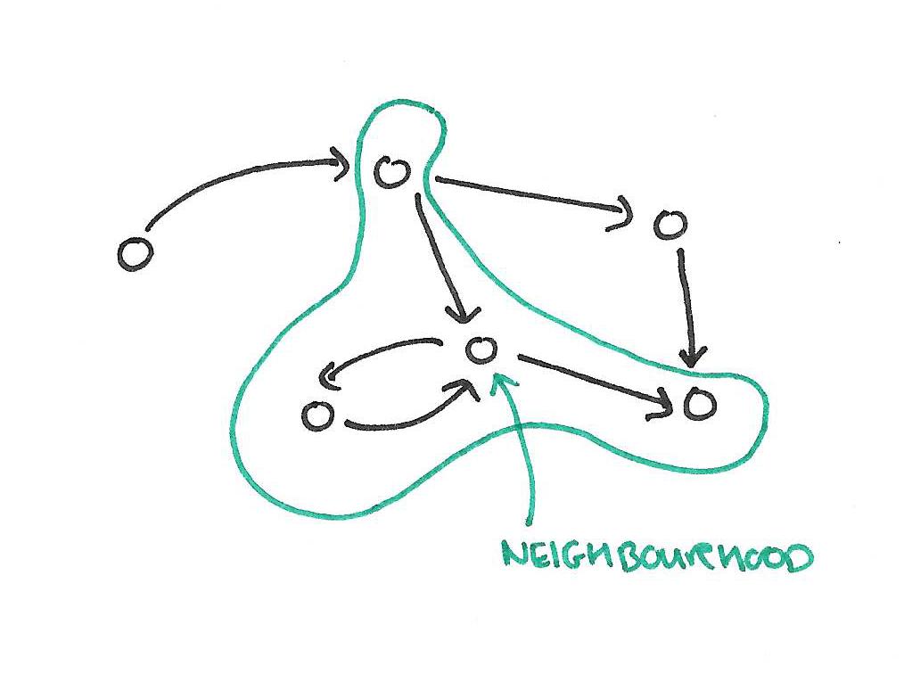
Of course, this means that neighbourhoods overlap. The consistency model determines what computations are allowed to proceed in parallel, and the scheduling model determines order of execution.
Sync Mechanism
The sync mechanism is similar to Pregel’s aggregators. For each aggregation (sync operation), the user supplies a key under which the result will be stored in the shared data table, a fold function, an apply function, and an optional merge function.
In the absence of a merge function, fold is applied sequentially to all vertices, and then the apply function is invoked on the result of the fold. If a merge function is provided, multiple folds can execute in parallel with merge being used to combine their results before the apply.
The sync mechanism can be set to run periodically in the background while the GraphLab engine is actively applying update functions or on demand triggered by update functions or user code. If the sync mechanism is executed in the background, the resulting aggregated value may not be globally consistent. Nonetheless, manyML applications are robust to approximate global statistics.
In the Loopy Belief Propagation example used in the paper, the sync mechanism is used to monitor the global convergence criterion.
Consistency Model
Since scopes may overlap, the simultaneous execution of two update functions can lead to race-conditions resulting in data inconsistency and even corruption… GraphLab provides a choice of three data consistency models which enable the user to balance performance and data consistency.
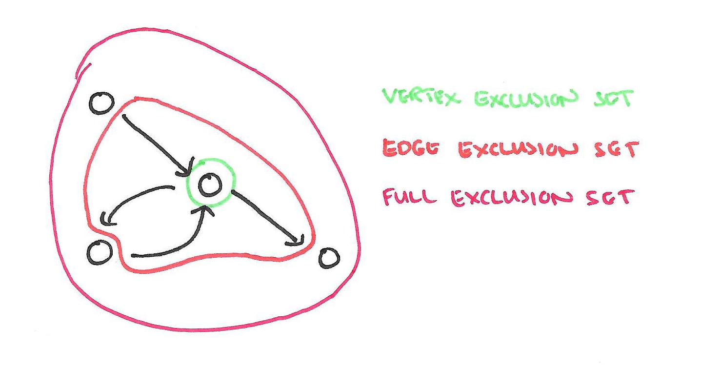
Each consistency model has a corresponding exclusion set.
GraphLab guarantees that update functions never simultaneously share overlapping exclusion sets. Therefore larger exclusion sets lead to reduced parallelism by delaying the execution of update functions on nearby vertices.
- The full consistency model treats an entire neighbourhood as an exclusion set.
- The edge consistency model protects a vertex and all of its incoming and outgoing edges (so parallel computation cannot occur for adjacent vertices).
- The vertex consistency model ensures only one function can operate on a given vertex at a time.
Scheduling
The GraphLab update schedule describes the order in which update functions are applied to vertices and is represented by a parallel data-structure called the scheduler. The scheduler abstractly represents a dynamic list of tasks (vertex-function pairs) which are to be executed by the GraphLab engine… To represent Jacobi style algorithms (e.g., gradient descent) GraphLab provides a synchronous scheduler which ensures that all vertices are updated simultaneously. To represent Gauss-Seidel style algorithms (e.g., Gibbs sampling, coordinate descent), GraphLab provides a round-robin scheduler which updates all vertices sequentially using the most recently available data.
GraphLab also provide task schedulers that allow update functions to add and reorder tasks.
GraphLab provides two classes of task schedulers. The FIFO schedulers only permit task creation but do not permit task reordering. The prioritized schedules permit task reordering at the cost of increased overhead. For both types of task scheduler GraphLab also provide relaxed versions which increase performance at the expense of reduced control… In addition GraphLab provides the splash scheduler based on the loopy BP schedule proposed by Gonzalez et al. which executes tasks along spanning trees.
In the Loopy Belief Propogation example, scheduler selection can be used to implement different variants of the algorithm. The synchronous scheduler corresponds to classic Belief Propogation, and the priority scheduler corresponds to Residual Belief Propagation.
Finally, GraphLab’s set scheduler enables users to safely and easily compose update schedules.
Case Studies
To demonstrate the expressiveness of the GraphLab abstraction and illustrate the parallel performance gains it provides, we implement four popular ML algorithms and evaluate these algorithms on large real-world problems using a 16-core computer with 4 AMD Opteron 8384 processors and 64GB of RAM.
The algorithms are: Markov Random Fields, Gibbs Sampling, Co-EM (a semi-supervised algorithm for Named Entity Recognition), and two different algorithms for Lasso. The programming model proved sufficient to express parallel solutions for all of these algorithms, and speed-ups of between 2x-16x were observed (most commonly one order of magnitude).
For the Co-EM example, we have a comparison between a single machine running GraphLab (16 cores), and a distributed Hadoop setup using 95 cores.
With 16 parallel processors, we could complete three full Round-robin iterations on the large dataset in less than 30 minutes. As a comparison, a comparable Hadoop implementation took approximately 7.5 hours to complete the exact same task, executing on an average of 95 cpus. [Personal communication with Justin Betteridge and Tom Mitchell, Mar 12, 2010]. Our large performance gain can be attributed to data persistence in the GraphLab framework. Data persistence allows us to avoid the extensive data copying and synchronization required by the Hadoop implementation of MapReduce.

6 thoughts on “GraphLab: A new framework for parallel machine learning”
Comments are closed.