The case for a learned sorting algorithm, Kristo, Vaidya, et al., SIGMOD’20
We’ve watched machine learning thoroughly pervade the web giants, make serious headway in large consumer companies, and begin its push into the traditional enterprise. ML, then, is rapidly becoming an integral part of how we build applications of all shapes and sizes. But what about systems software? It’s earlier days there, but ‘The case for learned index structures’(Part 1 Part 2), SageDB and others are showing the way.
Today’s paper choice builds on the work done in SageDB, and focuses on a classic computer science problem: sorting. On a 1 billion item dataset, Learned Sort outperforms the next best competitor, RadixSort, by a factor of 1.49x. What really blew me away, is that this result includes the time taken to train the model used!
The big idea
Suppose you had a model that given a data item from a list, could predict its position in a sorted version of that list. 0.239806? That’s going to be at position 287! If the model had 100% accuracy, it would give us a completed sort just by running over the dataset and putting each item in its predicted position. There’s a problem though. A model with 100% accuracy would essentially have to see every item in the full dataset and memorise its position – there’s no way training and then using such a model can be faster than just sorting, as sorting is a part of its training! But maybe we can sample a subset of the data and get a model that is a useful approximation, by learning an approximation to the CDF (cumulative distribution function).
If we can build a useful enough version of such a model quickly (we can, we’ll discuss how later), then we can make a fast sort by first scanning the list and putting each item into its approximate position using the model’s predictions, and then using a sorting algorithm that works well with nearly-sorted arrays (Insertion Sort) to turn the almost-sorted list into a fully sorted list. This is the essence of Learned Sort.
A first try
The base version of Learned Sort is an out-of-place sort, meaning that it copies the sorted elements into a new destination array. It uses the model to predict the slot in the destination array for each item in the list. What should happen though if the model predicts (for example) slot 287, but there’s already an entry in the destination array in that slot? This is a collision. The candidate solutions are:
- Linear probing: scan the array for nearest vacant slot and put the element there
- Chaining: use a list or chain of elements for each position
- A Spill bucket: if the destination slot is already full, just put the item into a special spill bucket. At the end of the pass, sort and merge the spill bucket with the destination array.
The authors experimented with all three, and found that the spill bucket approach worked best for them.

The resulting performance depends on the quality of the model predictions, a higher quality model leads to fewer collisions, and fewer out-of-order items to be patched in the final Insertion Sort pass. Since we’re punting on the details of the model for the moment, an interesting question is what happens when you give this learned sort a perfect, zero-overhead oracle as the model? Say we want to sort all the numbers from zero to one billion. A perfect zero-overhead oracle can be built by just using the item value as the position prediction. 1456? That will go in position 1456…
And what did happen when the authors tried to sort the numbers using this perfect zero-overhead oracle?
To our astonishment, in this micro-experiment we observed that the time take to distributed the keys into their final sorted position, despite a zero-overhead oracle function, took 38.7 sec and RadixSort took 37.5 sec.
Why? If it’s high performance you’re after, you can’t ignore mechanical sympathy. Radix Sort is carefully designed to make effective use of the L2 cache and sequential memory accesses, whereas Learned Sort is making random accesses all over the destination array.
Sympathy for the machine
How can learned sort be adapted to make it cache-efficient? The solution is to change the first pass of Learned Sort into a cascading Bucket Sort. Instead of determining the final position in the destination array, the model prediction is used to ascertain which bucket (or bin) the element should go into.
- Let
be the number of buckets (
is reached. If at any stage a model prediction places in an item in a bucket that is already full, this item is just moved to a spill bucket instead.
- Once we’re down to buckets of size
- Concatenate the sorted buckets in order (some may have less than elements in them), and use Insertion Sort to patch up any discrepancies in ordering.
- Sort and merge the spill bucket.
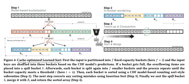
The secret to good performance with Learned Sort is choosing
The parameter
With these changes in place, if the number of elements to sort is close to the key domain size (e.g. sorting 2^32 elements with 32-bit keys), then Learned Sort performs almost identically to Radix Sort. But when the number of elements is much smaller than the key domain size, Learned Sort can significantly outperform Radix Sort.
Oh, yes – about the model!
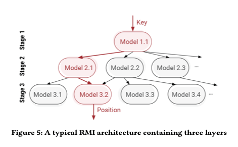
All of this depends of course on being able to train a sufficiently accurate model that can make sufficiently fast predictions, so that the total runtime for Learned Sort, including the training time still beats Radix Sort. For this, the authors use the Recursive Model Index (RMI) architecture as first introduced in ‘The case for learned index structures‘. In brief, RMI uses layers of simple linear models arranged in a hierarchy a bit like a mixture of experts.
During inference, each layer of the model takes the key as an input and linearly transforms it to obtain a value, which is used as an index to pick a model in the next layer.
The main innovation the authors introduce here is the use of linear spline fitting for training (as opposed to e.g. linear regression with an MSE loss function). Spline fitting is cheaper to compute and gives better monotonicity (reducing the time spent in the Insertion Sort phase). Each individual spline model fits worse than its closed-form linear regression counterpart, but the hierarchy compensates. Linear splines result in 2.7x faster training, and up to 35% fewer key swaps during Insertion Sort.
Evaluation
On synthetic datasets containing double-precision keys following a standard normal distribution, the authors compared Learned Sort to a variety of cache-optimized and highly tuned C++ implementations of alternative sorting algorithms, presenting the most competitive alternatives in their results. The following chart shows sorting rates over input dataset sizes varying from one million to one billion items.
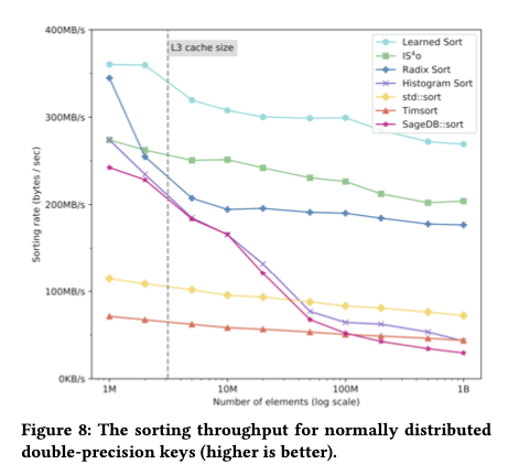
Learned Sort outperforms the alternative at all sizes, but the advantage is most significant when the data no longer fits into the L3 cache – an average of 30% higher throughput than the next best algorithm.
The results show that our approach yields an average 3.38x performance improvement over C++ STL sort, which is an optimized Quick- sort hybrid, 1.49x improvement over sequential Radix Sort, and 5.54x improvement over a C++ implementation of Tim- sort, which is the default sorting function for Java and Python.
Learned Sort’s advantage holds over real datasets as well (§6.1 for datasets included in the test), and for different element types:
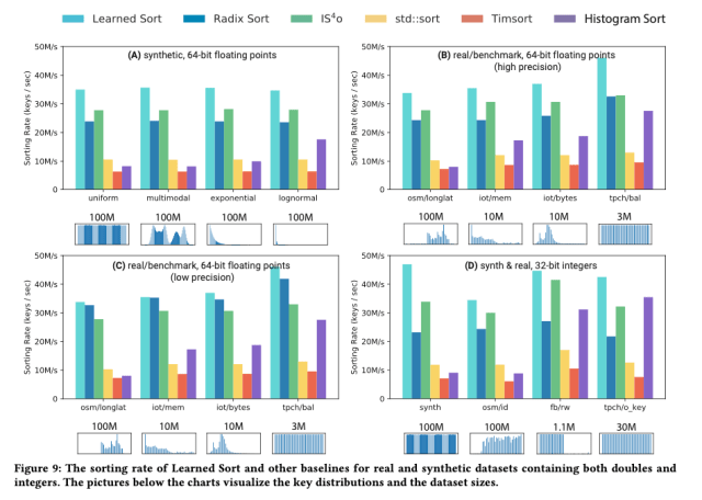
[Learned Sort] results in significant performance improvements as compared to the most competitive and widely used sorting algorithms, and marks an important step into building ML-enhanced algorithms and data structures.
Extensions
The paper also describes several extensions to Learned Sort including sorting in-place, sorting on other key types (strings initially), and improving performance for datasets with many duplicate items.
