Optimized risk scores Ustun & Rudin, KDD’17
On Monday we looked at the case for interpretable models, and in Wednesday’s edition of The Morning Paper we looked at CORELS which produces provably optimal rule lists for categorical assessments. Today we’ll be looking at RiskSLIM, which produces risk score models together with a proof of optimality.
A risk score model is a a very simple points-based system designed to be used (and understood by!) humans. Such models are widely used in e.g. medicine and criminal justice. Traditionally they have been built by panels of experts or by combining multiple heuristics . Here’s an example model for the CHADS2 score assessing stroke risk.
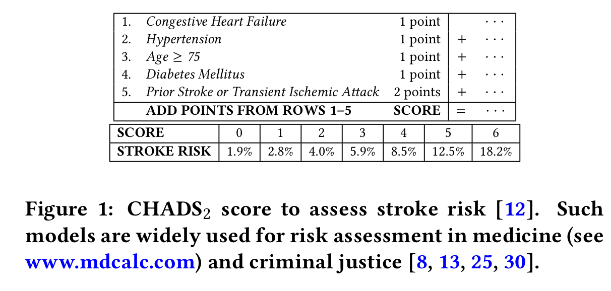
Even when you don’t consider interpretability as a goal (which you really should!), “doing the simplest thing which could possibly work” is always a good place to start. The fact that CORELS and RiskSLIM come with an optimality guarantee given the constraints fed to them on model size etc. also means you can make informed decisions about model complexity vs performance trade-offs if a more complex model looks like it may perform better. It’s a refreshing change of mindset to shift from “finding an approximation which seems to work ok,” to “solving for the optimal approximation given the constraints” too.
What makes a good risk model?
To keep the model easy to use, we’d like it to have a limited number of features and to use small integer coefficients, e.g. in the range -5 to 5. Moreover, we’d like to be able to specify additional operational constraints such as those shown in the table below.
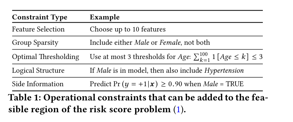
Using a limited number of features means that we’re looking for what is known as a sparse model. Using integer coefficients in a linear regression format means that we’re building a linear integer model. That’s where the RiskSLIM name comes from: the Risk-calibrated Supersparse Linear Integer Model. Solving such problems is the domain of MINLP (Mixed-Integer Non-Linear Programming).
What’s so hard about that?!
Optimizing RiskSLIM-MINLP is a difficult computational task given that
-regularization, minimizing over integers, and MINLP problems are all NP-hard. These worst-case complexity results mean that finding an optimal solution to RiskSLIM-MINLP may be intractable for high dimensional datasets.
But fear not, with a few optimisations RiskSLIM can be solved to optimality for many real-world datasets in minutes…
Cutting planes
There are off-the-shelf MINLP solvers, but used directly they take too long on this problem. The first step to make things more tractable is to introduce a cutting plane algorithm. Cutting plane algorithms (CPAs)”reduce data-related computation by iteratively solving a surrogate problem with a linear approximation of the loss that is much cheaper to evaluate.”
Suppose for a moment that we have a convex loss function (we can’t actually guarantee that, but we’ll get to what to do about it in the next section). The idea behind cutting-plane algorithms is to take successive piecewise linear approximations to the true loss function based on increasing the number of cuts. A picture helps. Here’s a cutting plane approximation with two cuts:
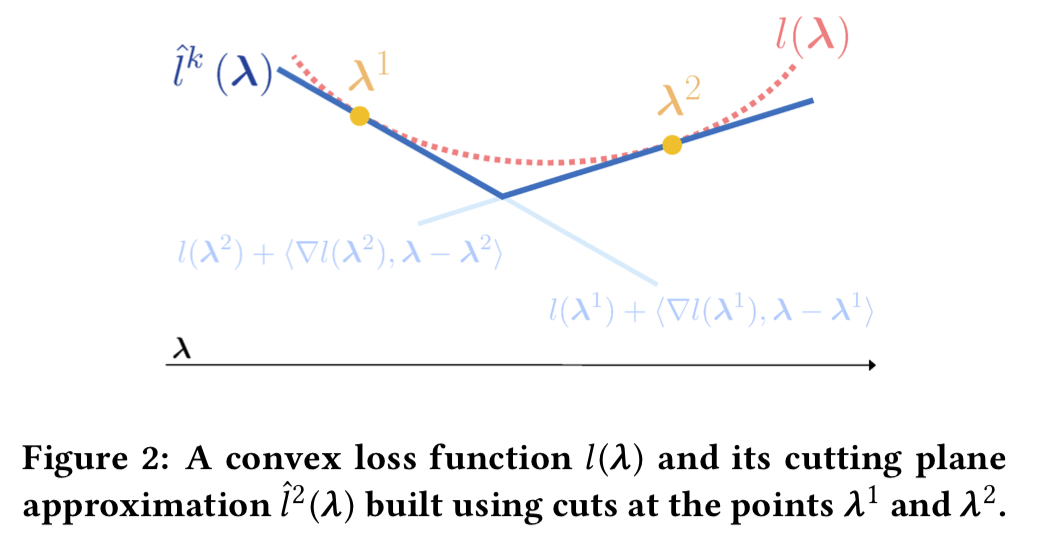
Each additional cut we add refines the approximation.
Since the cuts at each iteration are not redundant, the lower-bound improves monotonically as CPA progresses.
Now that we’re using cuts, the problem has become linear instead of non-linear, so we can use an MIP solver instead of a MINLP solver. “This can substantially improve our ability to solve RiskSLIM-MINLP since MIP solvers typically exhibit better off-the-shelf performance than MINLP solvers.”
The stalling problem
So far so good, but we have one remaining problem: the loss function we want to optimise is not guaranteed to be convex.
When (CPA) algorithms are applied to problems with non-convex regularizers or constraints, the surrogate problems are non-convex and may require an unreasonable amount of time to solve to optimality (especially on higher-dimensional problems). In practice, this prevents the algorithm from improving the cutting-plane approximation and computing a valid lower bound. We refer to this behavior as stalling.
The Lattice cutting plane algorithm (LCPA)
To avoid issues related to stalling, the authors introduce a variant of cutting-plane algorithms called a Lattice Cutting Plane Algorithm (LCPA).
LCPA is a cutting-plane algorithm that recovers the optimal solution to RiskSLIM-MINLP via branch-and-bound (B&B) search. The search recursively splits the feasible region of RiskSLIM-MINLP into disjoint partitions, discarding partitions that are infeasible or provably suboptimal. LCPA solves a surrogate linear program (LP) over each partition.
In practice, LCPA is implemented using a MIP solver that provides control callbacks, for example, CPLEX. In the algorithm below, a control callback is used to intervene at step 6. The callback computes the cut parameters, adds a cut, and returns control to the solver at step 9.
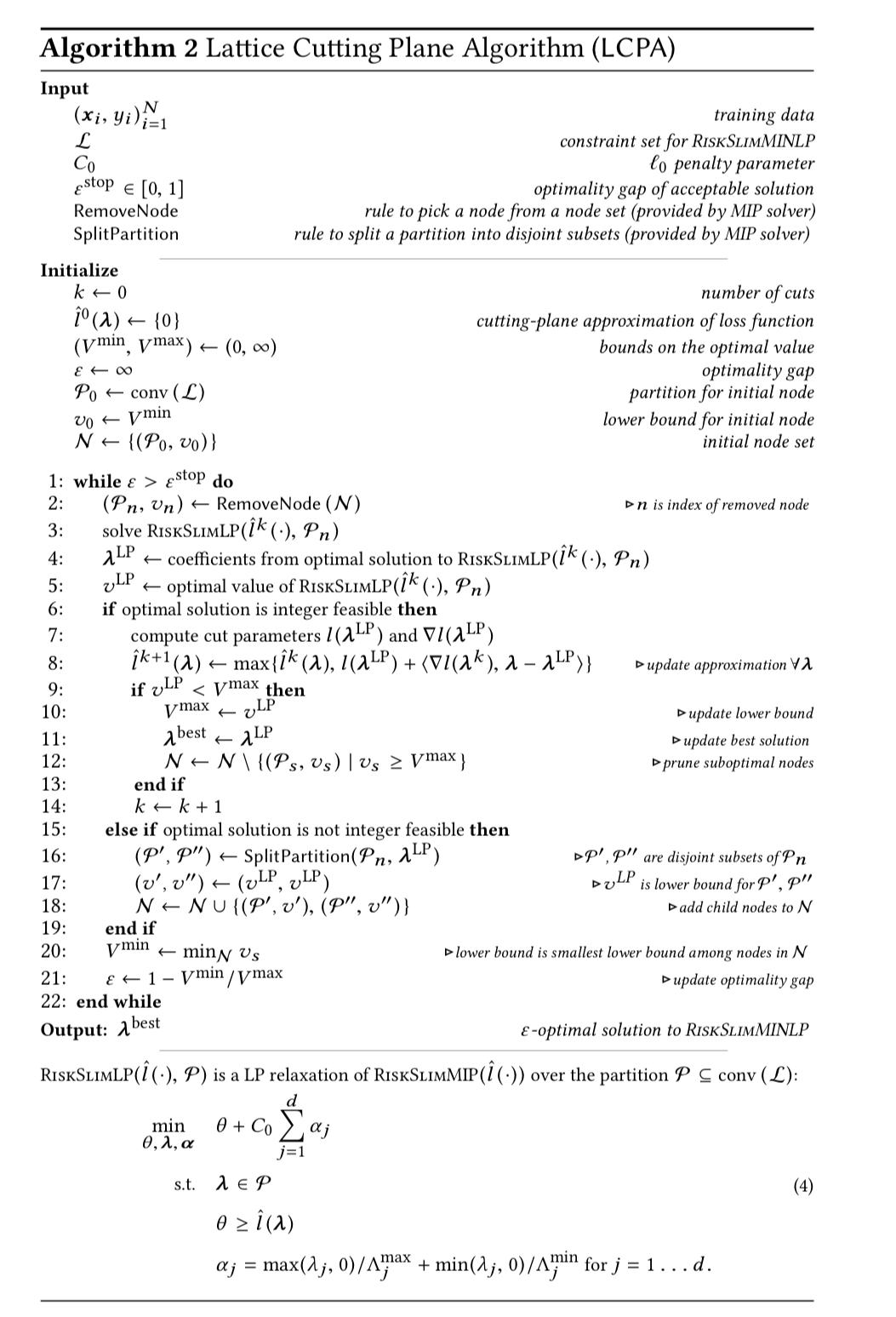
If that all looks a bit complicated, you can find a Python implementation on GitHub at https://github.com/ustunb/risk-slim.
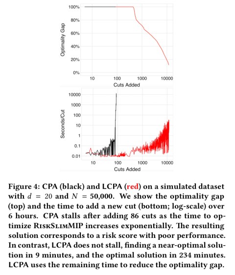
Here’s a comparison of standard CPA and LCPA on a simulated dataset in which you can clearly see CPA stalling after 86 cuts whereas LCPA finds a near-optimal solution in only 9 minutes.
RiskSLIM in action
RiskSLIM is evaluated across six different datasets, with models evaluated using risk-calibration (CAL) and rank accuracy (AUC). Compared to Penalised Logistic Regression (PLR), Naive Rounding (RD) and Rescaled Rounding (RSRD), the RiskSLIM models have the best CAL on 6/6 datasets and the best test AUC on 5/6 datasets.
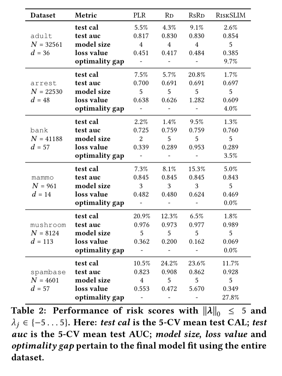
It takes RiskSLIM less than 20 minutes to find models with small optimality gaps in all cases. Bear in mind there is no need for parameter tuning etc. here, so to find these six models RiskSLIM just had to fit six models. The baseline methods required training and processing over 33,000 models!
RiskSLIM is the only method to pair models with a measure of optimality. In practice, small optimality gaps are valuable because they suggest we have fit the best model in our model class. Thus, if a risk score with a small optimality gap performs poorly, we can attribute the poor performance to a restrictive model class and improve performance by considering models with more terms or larger coefficients.
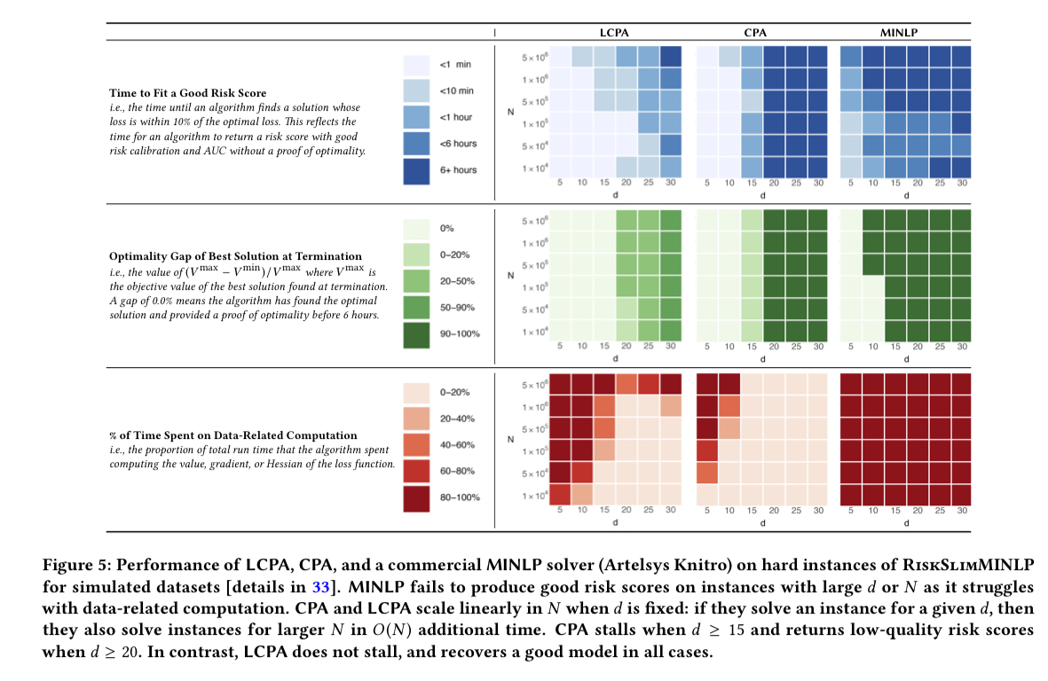
The charts below demonstrate the contribute of LCPA to finding models with small optimality gaps in reasonable time.
One additional thing I very much appreciate about these models is that when it comes time to put them into production (assuming they’re not going to be used by a human scorer) there’s no need for complex model serving platforms etc., I can just code up the scoring function in a simple method and be done! Easy to understand, easy to code, easy to review, and super-fast :).
This is really great, thanks for sharing! Checking out their GitHub.