DDSketch: a fast and fully-mergeable quantile sketch with relative-error guarantees Masson et al., VLDB’19
Datadog handles a ton of metrics – some customers have endpoints generating over 10M points per second! For response times (latencies) reporting a simple metric such as ‘average’ is next to useless. Instead we want to understand what’s happening at different latency percentiles (e.g p99).
The ability to compute quantiles over aggregated metrics has been recognized to be an essential feature of any monitoring system… Given how expensive calculating exact quantiles can be for both storage and network bandwidth, most monitoring system will compress the data into sketches and compute approximate quantiles.
Fortunately there are plenty of quantile sketching algorithms available including the GK-sketch, the t-digest, the HDR histogram, and the Moments sketch that we looked at last year. For reasons we’ll see shortly though, none of those were good enough for Datadog, so they developed their own sketching data structure, DDSketch. Officially in the paper DDSketch stands for ‘Distributed Distribution Sketch’ but that seems a bit of a stretch… surely it’s the ‘Datadog Sketch’ ! A glance at the code repository for the Python implementation confirms my suspicion: there are several references to ‘DogSketch’ in the commit history and the codebase still ;).
In putting together this write-up I’m grateful to the first author, Charles Masson, who gave a great talk on this paper at the VLDB conference and was kind enough to share his slides with me. Some of the images in this post are taken from Charles’ slide deck with permission.
Why do we need a new sketch?
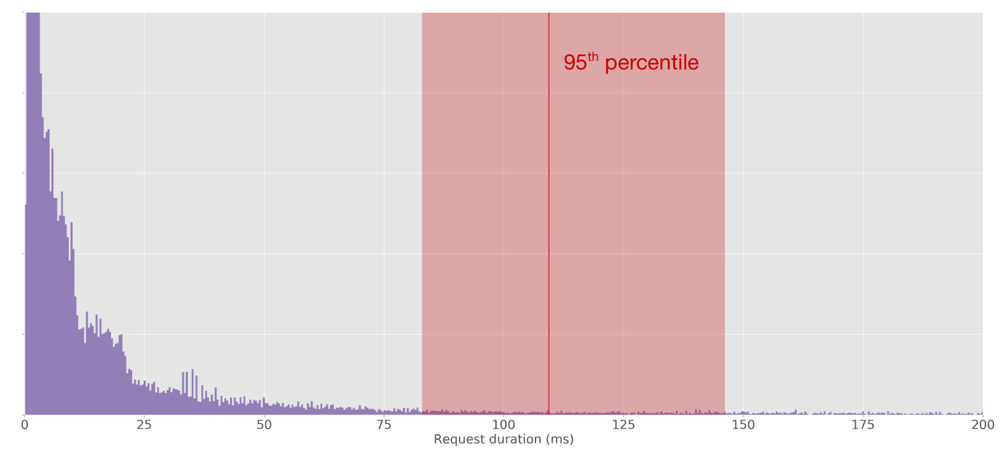
A characteristic of latency distributions is that they have a long tail. This can play havoc with quantile sketches that are based on rank error. At the 50th percentile, an accuracy within 0.5% is still pretty tightly bound in absolute terms. But the further out into the tail we go, the more spread apart things get:
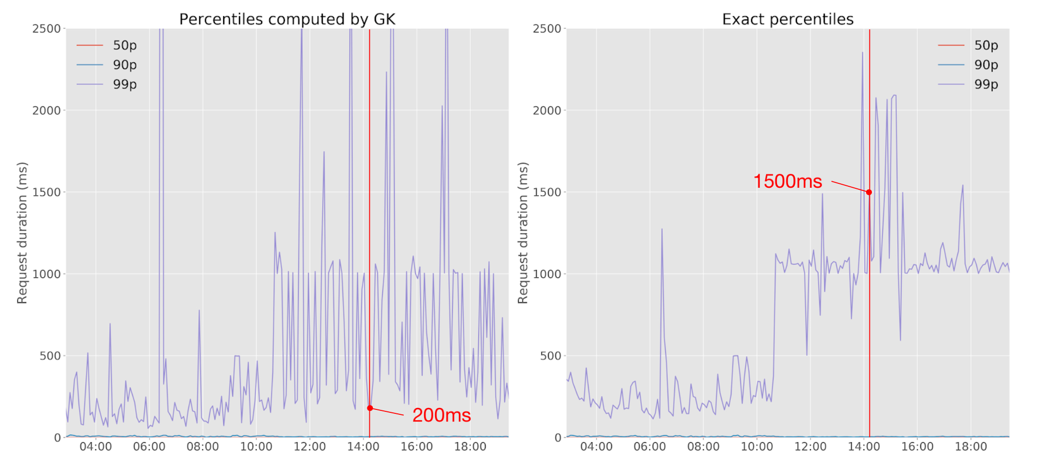
In this example, you can see that the GK-sketch, which uses rank error, is out by 1300ms compared to the ground truth. And look how noisy the sketch is!
In another example in the paper, a rank accuracy of 0.5% at the 99%-ile guarantees us a value between the 98.5th and 99.5th percentiles…
In this case, this is anywhere from 2 to 20 seconds, which from an end user’s perspective is the difference between an annoying delay and giving up on the request.
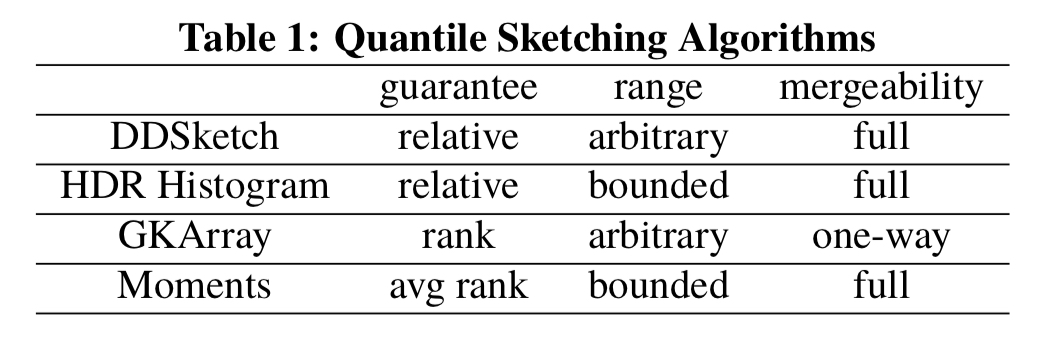
t-digest sketches are also rank based, but give lower errors on quantiles further away from the medium than uniform rank-error sketches. But even so, the error is still relatively high on heavily-tailed datasets.
The HDR Histogram uses relative error, which retains accuracy into the tail (you’d expect nothing less from it’s creator, Gil Tene, who surely knows a thing or two about performance analysis!). Its two weaknesses are that it can only handle a bounded (but large!) range, and that it has no published guarantees.
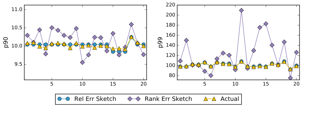
The Moments sketch only guarantees it’s accuracy for the average rank error (not the worst case).
We want a fast-to-insert, fully mergeable (we can combine sketches in a distributed manner), space-efficient quantile sketch with relative error guarantees. So it looks like we’re going to need a new sketch!
How DDSketch works
First let’s define what we mean by relative error. An α-accurate -sketch outputs quantiles within
of the true value
for all quantiles
,
. E.g., if α is 1%, then we’ll be within 1% of the true value.
The basic version of the sketch gives (0,1) α-accurate sketches (i.e. they’re accurate over the full range). We’re going to divide response times into buckets, and count the number of points that fall into each bucket. The trick is to assign the bucket sizes (boundaries) such that when we compute quantiles using the bucket counts we retain the desired accuracy.
Let . So for
we have
.
Bucket will be used to store values between
and
. In practical terms, when we see a value
we take
and round up to the nearest whole number to get the bucket number. Then we just increment the counter for that bucket.

Insertion is therefore relatively fast, and merging two sketches with the same is as simple as summing up bucket counts by index.
Now, when we want to know the estimate of the qth quantile we add up the bucket counts until we find the bucket containing the qth quantile value. With n total elements counted, it looks like this:
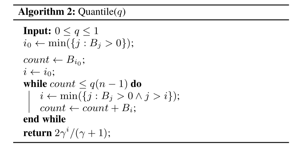
However buckets are stored in memory (e.g., as a dictionary that maps indices to bucket counters, or as a list of bucket counters for contiguous indices), the memory size of the sketch is at least linear in the number of non-empty buckets.
So given a pathological input of n points each falling into a different bucket, we have worse case size O(N). To keep a bound on the size we can make one small tweak, yielding the the full DDSketch in all its glory:
The full version of DDSketch is a simple modification that addresses its unbounded growth by imposing a limit of
on the number of buckets it keeps track of. It does so by collapsing the buckets for the smallest indices:
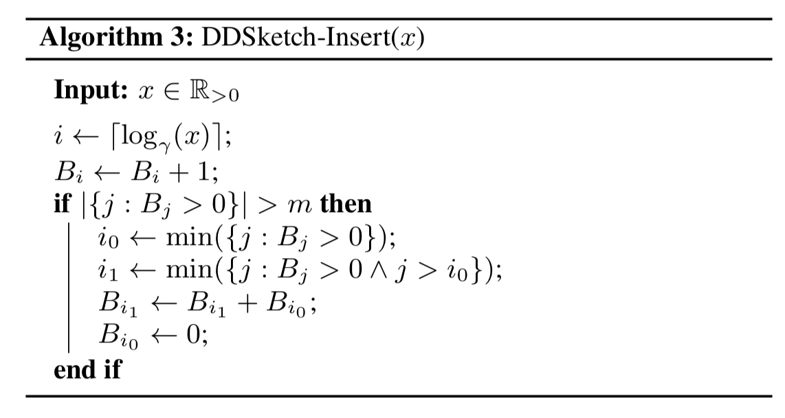
When we merge two sketches that have both independently kept their number of buckets within the limit, we might end up with more buckets than we wanted. So we do the same bucket collapsing trick on merging as well to fix that.
The paper of course has proofs that all this provides the desired guarantees, but I’m just going to take their word for it ;).
For response times we don’t need to worry about negative values. But if you have a use case where you do, the solution is to keep one DDSketch for positive numbers, and another one for negative numbers.
DDSketch in action
How well does it work? How about this:
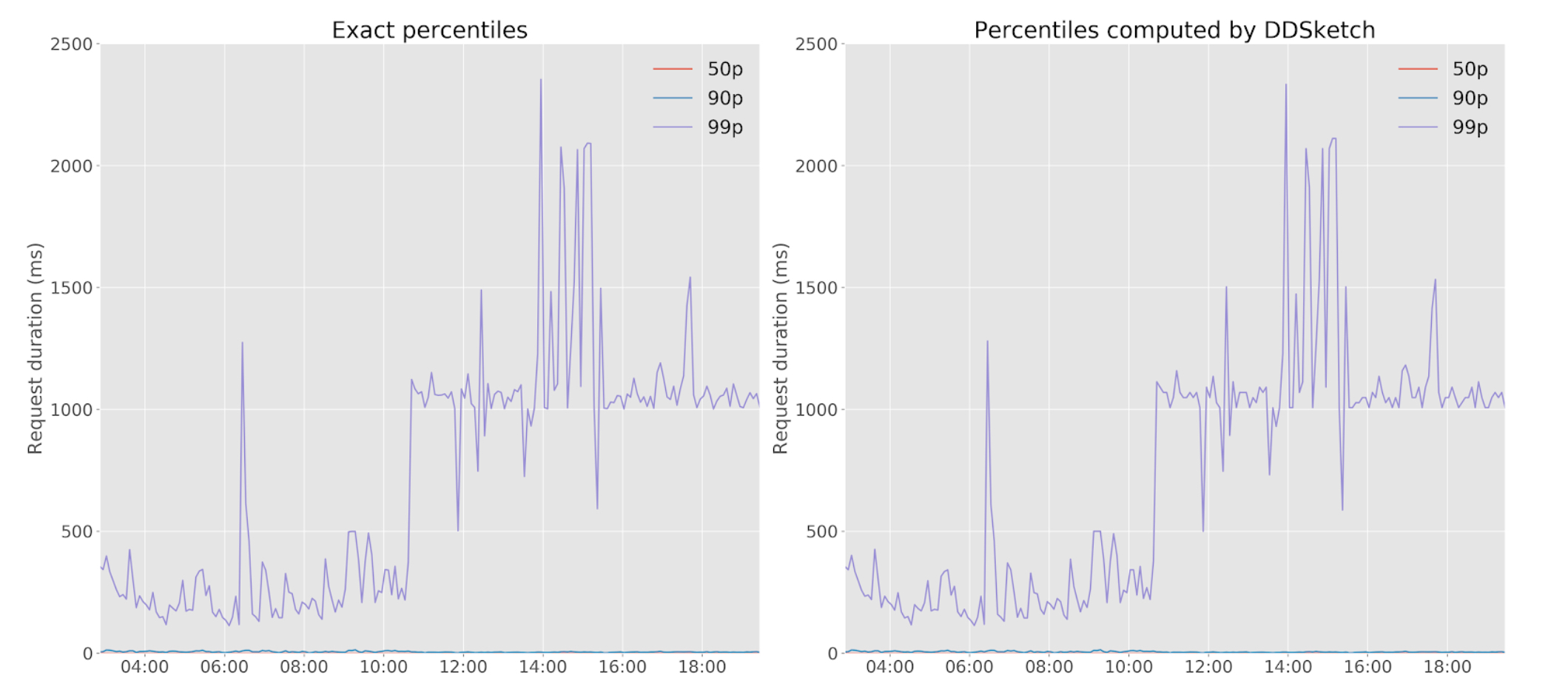
Beautiful tracking of the true values without any discernible noise :).
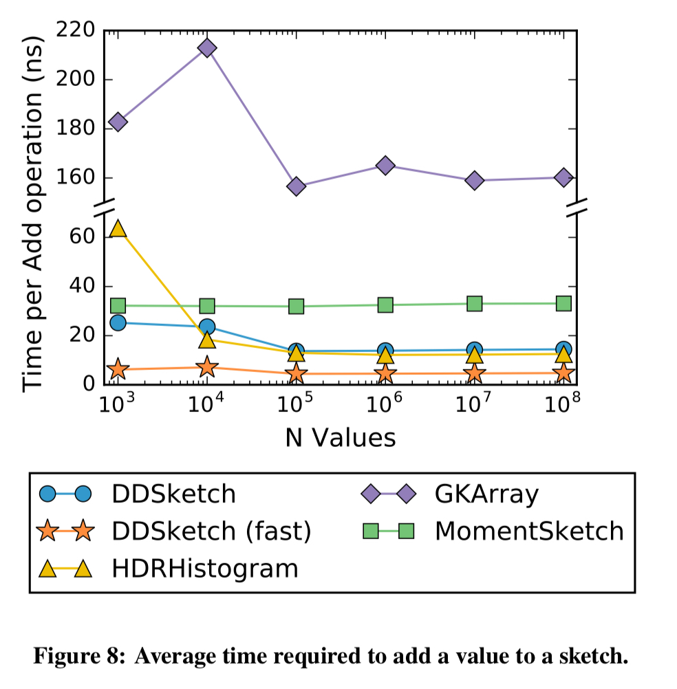
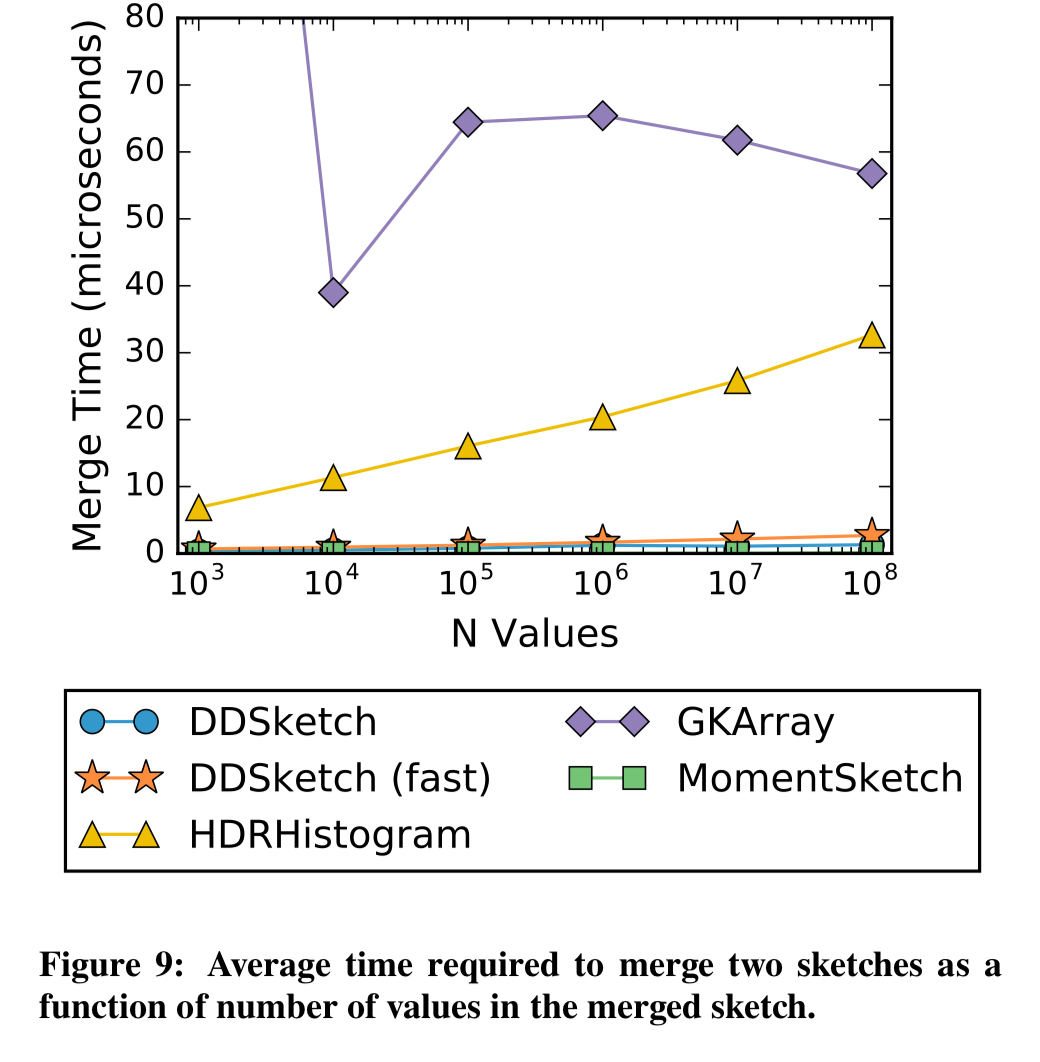
In the evaluation DDSketch (fast) stores buckets in a contiguous way for fast addition, and DDSketch (vanilla) stores buckets in a sparse way for smaller memory footprint.
DDSketch is pretty good in terms of memory usage:
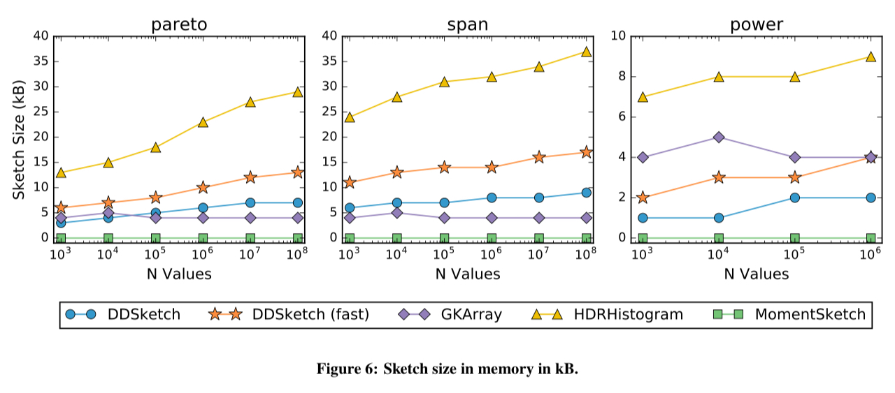
Has fast insert times:
And super-fast merges:
[DDSketch is] the first fully-mergeable, relative-error quantile sketching algorithm with formal guarantees. The sketch is extremely fast and accurate, and is currently being used by Datadog at a wide-scale.
Yes, the academic literature will probably continue to refer to it as the ‘Distributed Distribution’ sketch. But you and I can just call it the “Datadog” sketch :). The kind folks at Datadog have even open sourced implementations for you in Python, Go, and Java.
I would like to point out that the open source implementation does not use Algorithm 1 for mapping values to buckets by default. Instead, the standard factory method creates a DDSketch that uses a mapping based on a quadratic approximation of the logarithm function which preserves the same relative error guarantees using only little more space. I have already proposed this mapping a couple of years ago as improvement to HdrHistogram (see https://github.com/HdrHistogram/HdrHistogram/issues/54). The corresponding code (see https://github.com/oertl/HdrHistogram/blob/memory_efficiency/src/main/java/org/HdrHistogram/MemoryEfficientHistogram.java) is almost the same as in the DDSketch library (see https://github.com/DataDog/sketches-java/blob/master/src/main/java/com/datadoghq/sketch/ddsketch/mapping/QuadraticallyInterpolatedMapping.java). On Hacker News, where this paper was promoted (see https://news.ycombinator.com/item?id=20829404), the authors admitted that they had been aware of my proposal. Unfortunately, this is neither mentioned in the paper nor in the published source code.