Neural ordinary differential equations Chen et al., NeurIPS’18
‘Neural Ordinary Differential Equations’ won a best paper award at NeurIPS last month. It’s not an easy piece (at least not for me!), but in the spirit of ‘deliberate practice’ that doesn’t mean there isn’t something to be gained from trying to understand as much as possible.
In addition to the paper itself, I found the following additional resources to be helpful:
- Thread on HN
- Kevin Gibson’s blog post on the paper
- Branislav Holländer’s post on ‘Towards Data Science
- Adam Kosiorek’s introduction to normalizing flows (as linked from the previous post)
- High level summary in MIT TR’s ‘The Algorithm’ newsletter
Neural networks as differential equations
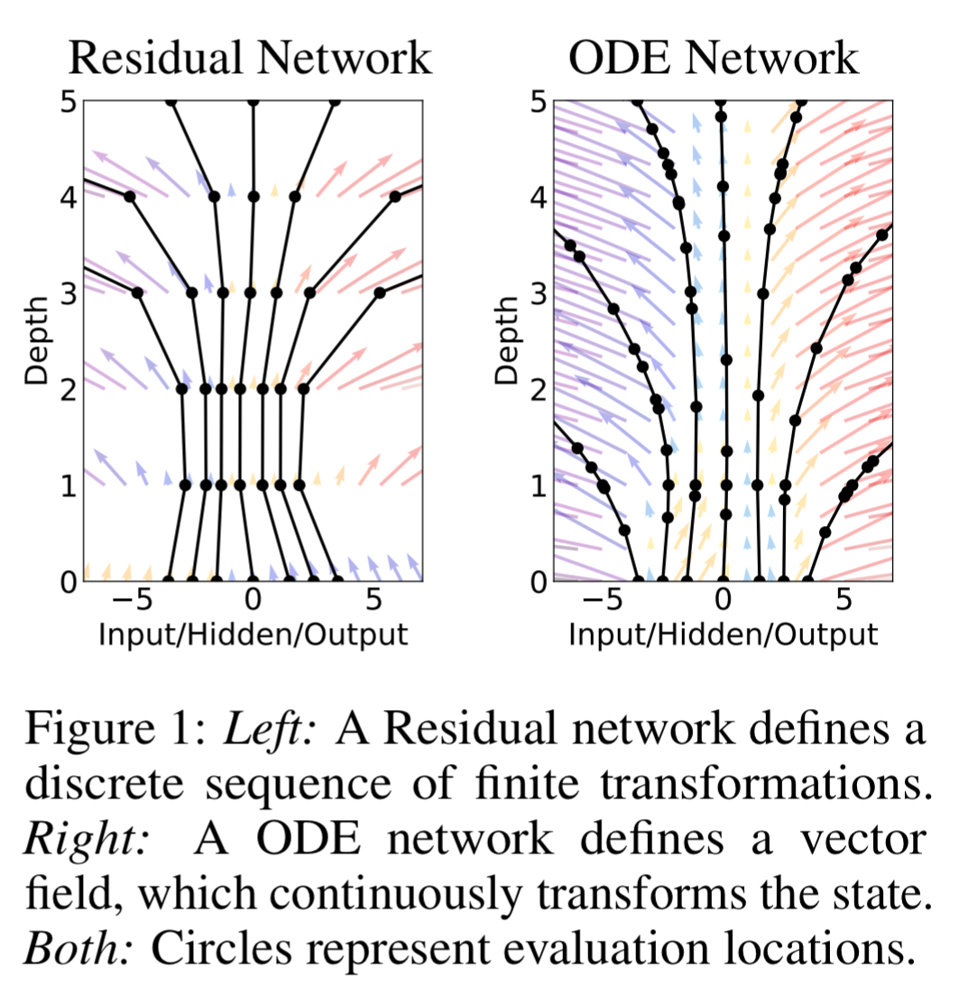
Consider a multi-layered neural network. We have an input layer and an output layer, and inbetween them, some number of hidden layers. As an input feeds forward through the network, it is progressively transformed, one layer at a time, from the input to the ultimate output. Each network layer is a step on that journey. If we take a small number of big steps, we end up with a rough approximation to the true transformation function we’d like to learn. If we take a much larger number of steps (deeper networks), with each step being individually smaller, we have a more accurate approximation to the true function. What happens in the limit as we take an infinite number of infinitely small steps? Calculus!
So one way of thinking about those hidden layers is as steps in Euler’s method for solving differential equations. Consider the following illustration from wikipedia:

We want to recover the blue curve, but all we have is an initial point 


Many neural networks have a composition that looks exactly like the steps of Euler’s method. We start with an initial state 
- …


In the limit, we parameterize the continuous dynamics of hidden units using an ordinary differential equation (ODE) specified by a neural network:

The equivalent of having T layers in the network, is finding the solution to this ODE at time T.
Something really neat happens once we formulate the problem in this way though. Just like we’ve seen a number of papers that express a problem in a form suitable for solving by a SAT solver, and then throw a state of the art SAT-solver at it, we can now use any ODE solver of our choice.
Euler’s method is perhaps the simplest method for solving ODEs. There since been more than 120 years of development of efficient and accurate ODE solvers. Modern ODE solvers provide guarantees about the growth of approximation error, monitor the level of error, and adapt their evaluation strategy on the fly to achieve the requested level of accuracy. This allows the cost of evaluating a model to scale with problem complexity.
How to train a continuous-depth network
We’ve seen how to feed-forward, but how do you efficiently train a network defined as a differential equation? The answer lies in the adjoint method (which dates back to 1962). Think of the adjoint as the instantaneous analog of the chain rule.
This approach computes gradients by solving a second, augmented ODE backwards in time, and is applicable to all ODE solvers. This approach scales linearly with problem size, has low memory cost, and explicitly controls numerical error.
The adjoint captures how the loss function L changes with respect to the hidden state ( 

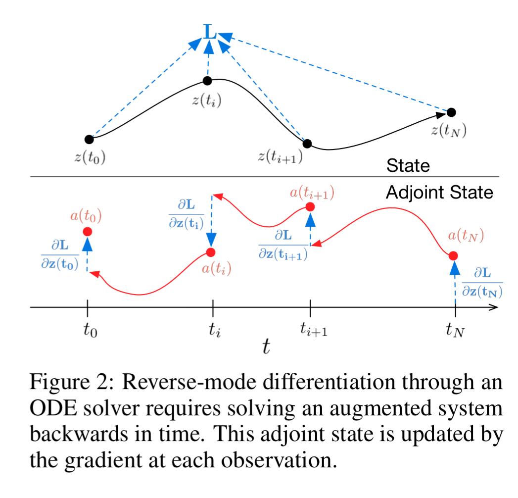
A third integral then tells us how the loss changes with the parameters 

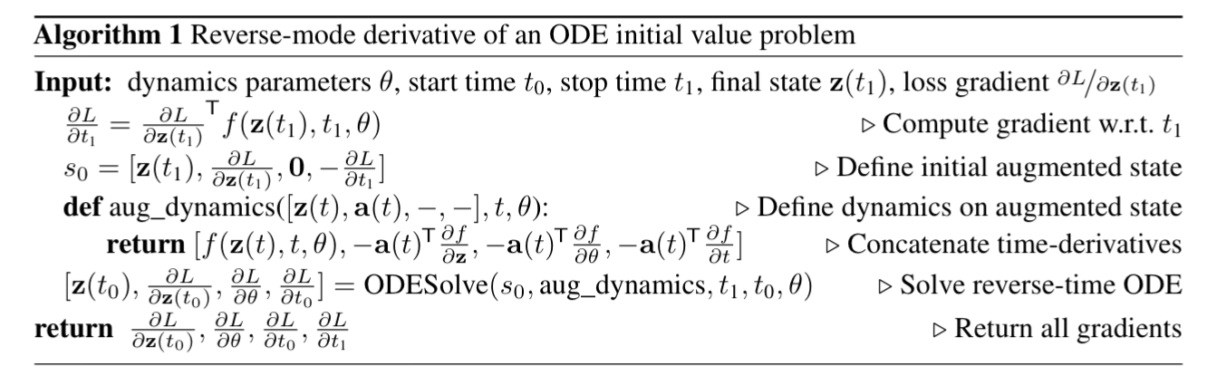
All three of these integrals can be computed in a single call to an ODE solver, which concatenates the original state, the adjoint, and the other partial derivatives into a single vector. Algorithm 1 shows how to construct the necessary dynamics, and call an ODE solver to compute all gradients at once.
(Don’t ask me to explain that further!)
Applied Neural ODEs
Residual Networks
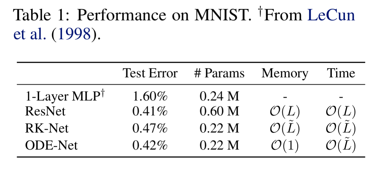
Section three tackles the good old MNIST problem, comparing an ODE-net to a ResNet with 6 residual blocks. The ODE-net replaces the residual blocks with an ODE-Solve module.
Concentrating on the 2nd and 4th lines in the table below, ODE-Nets are able to achieve roughly the same performance as a ResNet, but using only about 1/3 of the parameters. Also note that the ODE-Net solution using constant memory, whereas ResNets use memory proportional to the number of layers.
It’s not clear how to define the ‘depth’ of an ODE solution. A related quantity is the number of evaluations of the hidden state dynamics required, a detail delegated to the ODE solver and dependent on the initial state or input. The figure below shows the number of function evaluations increases throughout training, presumably adapting to increasing complexity of the model.
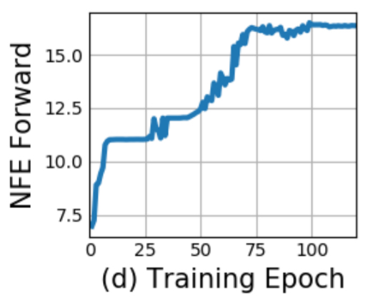
In other words, the ODE-net is kind of doing the equivalent of deepening its network over time as it needs to add sophistication.
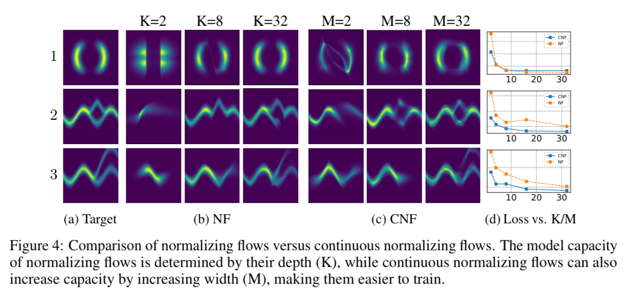
Normalising flows
Normalizing flows allow more complex probability distribution functions (pdfs) to be learned. The same trick of shifting from a discrete set of layers to a continuous transformation works in this situation too. The following figure shows normalising flows vs continuous normalising flows (CNF) when trying to learn a pdf. The CNF is trained for 10,000 iterations and generally achieves lower loss than the NF trained for 500,000 iterations.
Time-series
This is the application which most caught my attention.
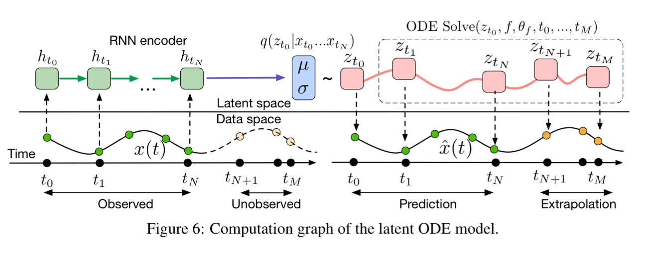
Applying neural networks to irregularly-sampled data such as medical records, network traffic, or neural spiking data is difficult. Typically, observations are put into bins of fixed duration, and the latent dynamics are discretized in the same way. This leads to difficulties with missing data and ill-defined latent variables… We present a continuous-time, generative approach to modeling time series. Our model represents each time series by a latent trajectory. Each trajectory is determined from a local initial state
, and a global set of latent dynamics shared across all time series.
The model can be trained as a variational autoencoder, and it looks like this:
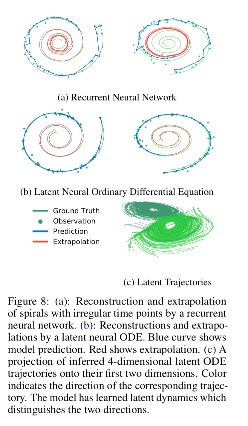
The evaluation here is based on a dataset of 1000 2-dimensional spirals, each starting at a different point. Half of the spirals are clockwise, and half counter-clockwise. Points are sampled from these trajectories at irregular timestamps. The figure below shows a latent neural ODE is better able to recover the spirals than a traditional RNN:
A PyTorch implementation of ODE solvers is available.

Thanks, Adrian! Applying NN to ODEs has similarities to Echo State Networks (Reservoir Computing). Any idea where to look for comparisons and resource requirements, and total cost benchmarks viz conventional ODE solvers?