Customized regression model for Airbnb dynamic pricing Ye et al., KDD’18
This paper details the methods that Airbnb use to suggest prices to listing hosts (hosts ultimately remain in control of pricing on the Airbnb platform).
The proposed strategy model has been deployed in production for more than 1 year at Airbnb. The launch of the first iteration of the strategy model yielded significant gains on bookings and booking values for hosts who have adopted our suggestions… multiple iterations of the strategy model have been experimented [with] and launched into production to further improve the quality of our price suggestions.
Figuring out the right price for a night in a given Airbnb listing is challenging because no two listings are the same. Even when we constrain to e.g. similar sized properties in the same region, factors such as the number of five star reviews can influence price. Furthermore demand is time-varying due to seasonality and regional events (with different seasonality patterns for different countries). And then of course, how far in advance a booking is being made also factors into the price (“as lead time reduces, there are less opportunities for this night to be booked, which leads to changes in the demand function“).
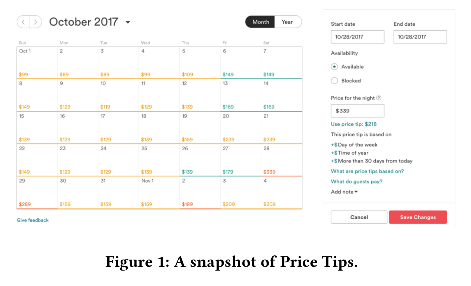
To help hosts maximise their revenues, Airbnb offers “Price Tips” and “Smart Pricing” tools. Price Tips presents a calendar view showing the predicted likelihood of bookings on a day-by-day basis, given the current pricing as set by the host. When clicking on a given day, more detail and an Airbnb suggested price are shown.
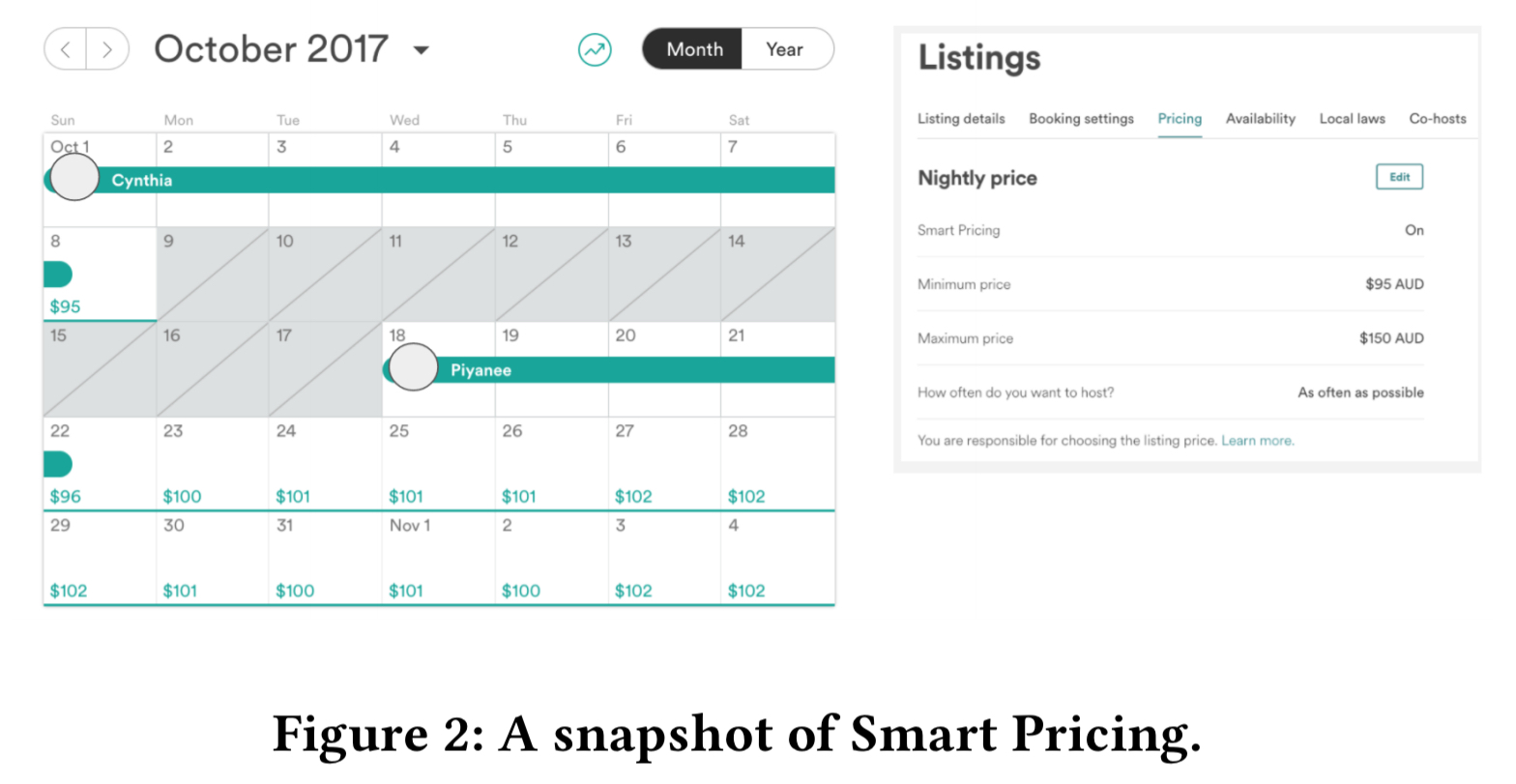
With Smart Pricing hosts can set a min and max price and then any new price suggestions generated by Airbnb that fall within these ranges will be automatically adopted for all available nights.
In the ideal world we’d estimate a demand curve F(P) giving an estimate of demand at a given price P, and then choose P so as to maximise 

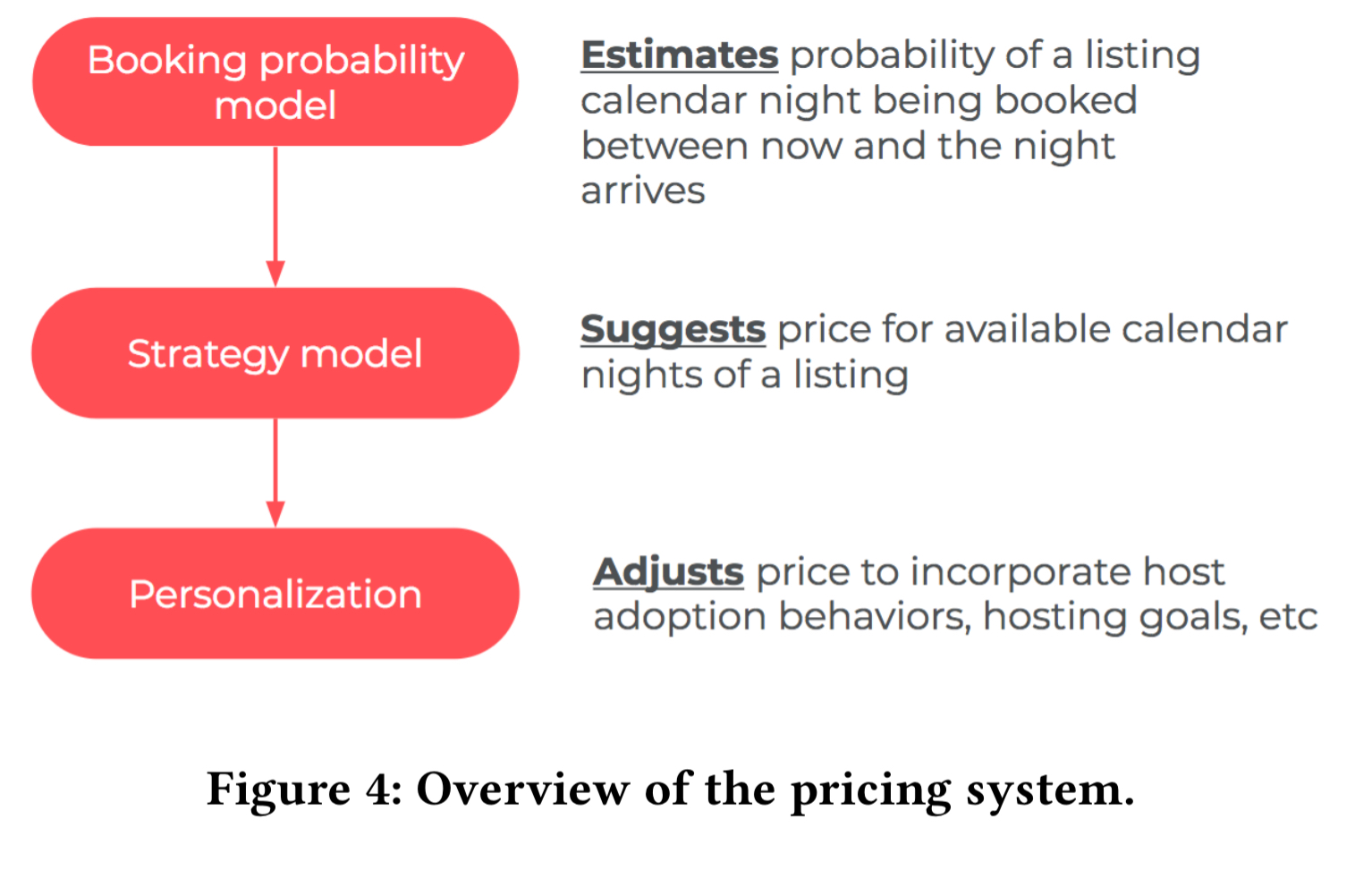
The pricing system that Airbnb ultimately settled on has three components:
- First a booking probability binary classification model makes predictions of the likelihood a listing will be booked on each night.
- These predictions are then fed into a pricing strategy model which suggests prices for the available nights
- Additional personalisation logic is applied to the prices output by the strategy model to incorporate hosting goals, special events etc..
The main focus of this paper is the pricing strategy model, but we do get brief details on the booking probability model.
The Booking probability model
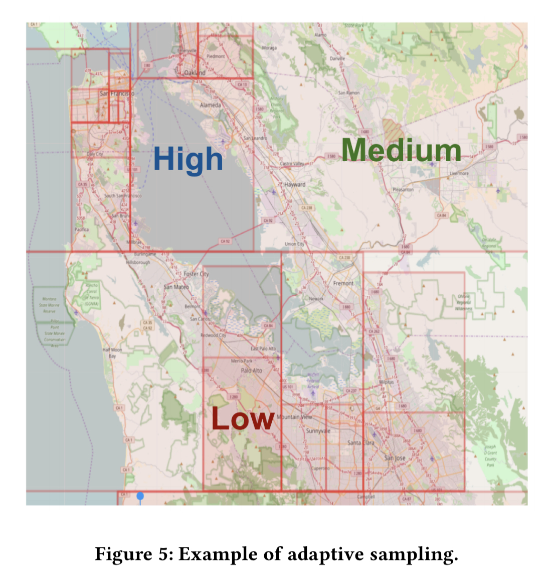
Booking probability is predicted using Gradient Boosting Machines (GBM), with a separate model trained for each market. The sampling rate for training data varies based on market density:
Markets with a high density of listings benefit from the location-based models the most, which we sample at a rate higher than the global constant sampling rate.
The models take into account three different types of features:
- Listing features such as listing price per night, room type, person capacity, number of bedrooms/bathrooms, amenities, locations, reviews, historical occupancy rate, whether or not instant booking is enabled, and so on.
- Temporal features such as seasonality (day of year, day of week etc.), calendar availability (gap between check-in and check-out), how many days there are between now and the night in question, and so on.
- Supply and demand features such as number of available listings in the neighbourhood, listing views, search / contact rates, and so on.
By scoring the booking probability model at different price points in a range it’s possible to get an estimated demand curve. However, due to the challenges outlined above getting an accurate enough demand curve at listing-night level to use for price setting is extremely difficult.
We have tried to directly apply revenue maximization strategies based on our estimated demand curve, but online A/B testing results showed that these methods often fail to optimize revenue for our hosts in practice. Therefore, we decide to pursue alternative solutions…
The alternative solution using the output of the booking probability model as just one input into the pricing strategy model.
The Pricing strategy model
Let’s start with this: in the absence of a ground truth for the optimal price, what should you use as an evaluation metric for training a pricing strategy model?
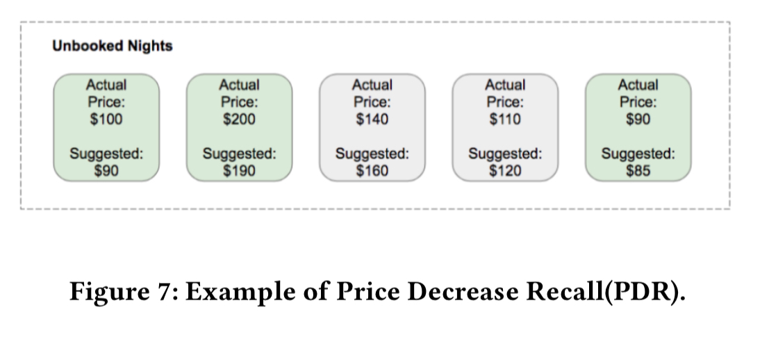
After some deliberation, the team settled on two evaluation metrics: price decrease recall (PDR) and booking regret (BR). We do have historical information on whether a given listing was actually booked on a given night, and the price it was booked at. Both PDR and BR tap into this information.
Let’s assume that if a listing wasn’t booked on a given night at price P, then it also wouldn’t have been booked at some suggested price ≥ P. But if the price had been lower than 
If all we had was PDR though, we’d end up training a model to offer free accommodation every night! If a listing was booked on a given night at some price P, and we suggest a price for the night ≤ P, then our suggestion is leaving money on the table. Booking Regret captures this missed revenue. BR is calculated as follows: for all the booked nights, take the maximum of zero and the percentage below the booked price of the suggested price. Now take the median of these values.
For example, given:
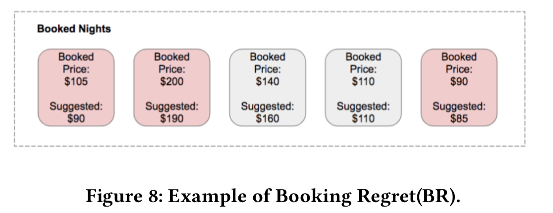
Then BR will be the median of (14, 5, 6, 0, 0) = 5%.
Now we need a way to combine these ideas into a single loss function. It looks like this:
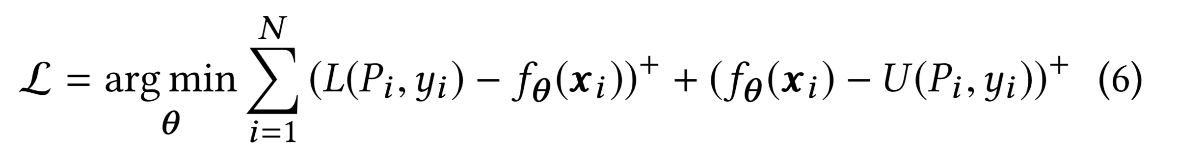
It’s not as bad as it looks, honest! 

For booked listing nights, the lower bound is the booking price 


For non-booked listing nights, the upper bound is the calendar price 

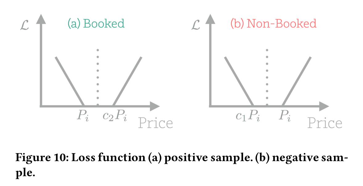
When suggestions fall between the upper and lower bound, the loss is zero; otherwise the loss is the distance between the suggestion and the bound.
The set of features 

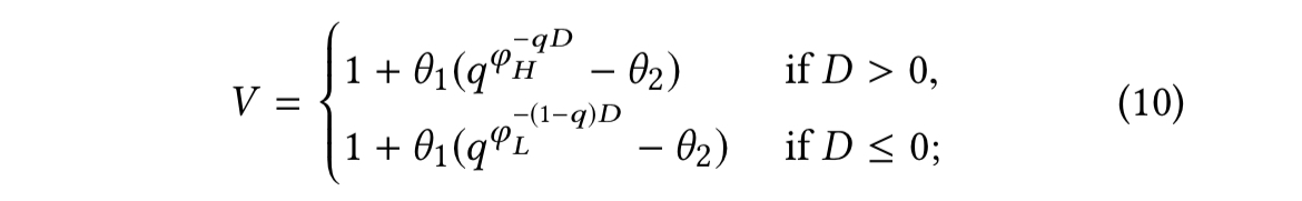
- D is a demand score computed from additional demand signals at the cluster level (a cluster is a group of similar listings).
controls how fast the prices grow/shrink
controls when the original calendar price is suggested
- q is the estimated booking probability
and
are constants between 1 and 2 which control the extent to which the suggestion curves bend.
We do not use the same constants for price increases and decreases since we would like the training system to learn the ratios asymmetrically. In this way, price suggestions can reflect the demand sensitivity more thoroughly by taking advantage of the non-linear manner in which markets perceive supply and demand.
The parameters
Evaluation
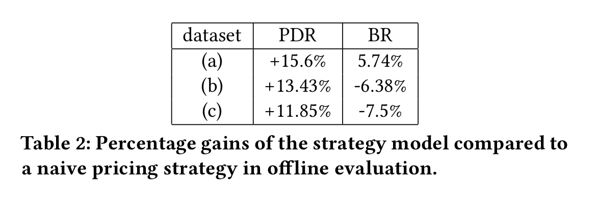
Offline and online evaluation results show that the proposed strategy model performs significantly better than a direct max-rev pricing strategy. We are also actively working on improving the demand curve estimation. With a more accurate demand curve, we may revisit the direct revenue maximization strategy in the future.
Compared to a naive strategy of pricing directly off of the demand estimation curves from the booking probability model, the pricing strategy model significantly improves PDR and BR (except for BR with dataset (a)).
As well as a quantitative evaluation (details in section 5.1 of the paper), the authors also inspected price suggestions generated on 2018-02-08 for 120 nights into the future. The following figures show the suggestions generated for Tokyo and for Tahoe respectively.
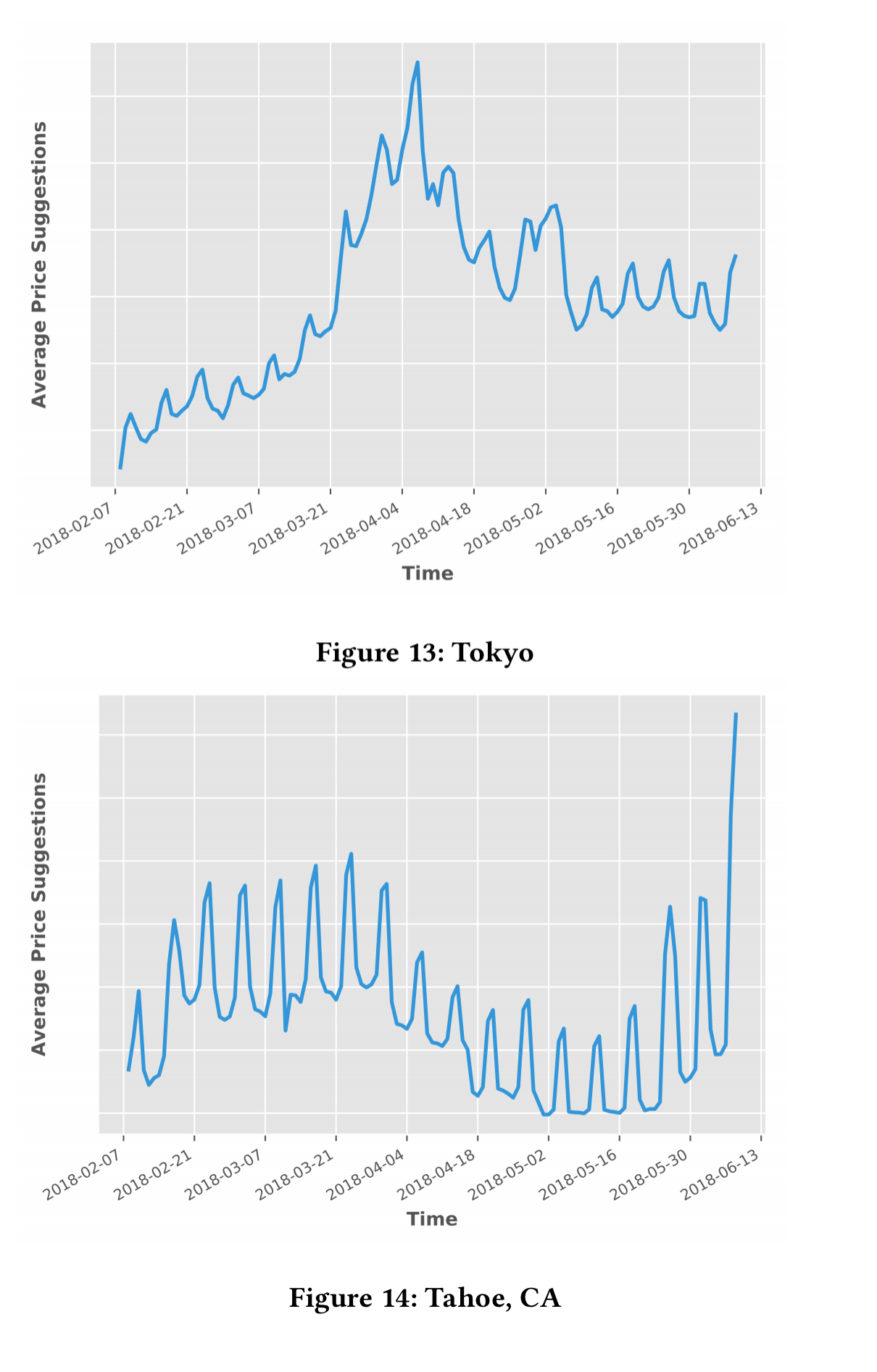
For both markets strong weekly patterns emerge, and in Tokyo there is also a strong spike from late March to early April corresponding with the cherry blossom season. “From these two examples, we see that our model can indeed capture the market dynamics in a timely fashion.“

Thank you for this great article.
You do not talk about the models used for “Additional personalisation logic is applied to the prices output by the strategy model to incorporate hosting goals, special events etc..”
Could you tell more about this?
Great read. The model looks good and shows that the system has a lot more opportunities to collect data about the behaviour of the cities. I would love to read more from you.