The design and implementation of modern column-oriented database systems Abadi et al., Foundations and trends in databases, 2012
I came here by following the references in the Smoke paper we looked at earlier this week. “The design and implementation of modern column-oriented database systems” is a longer piece at 87 pages, but it’s good value-for-time. What we have here is a very readable overview of the key techniques behind column stores.
What is a column store?
Column stores are relational databases that store data by column rather than by row. Whereas a traditional row-based store stores all attributes of one row together, followed by the attributes of the next row, and so on, a column-based stored uses one logical file per attribute (column). The column-oriented layout makes it efficient to read just the columns you need for a query, without pulling in lots of redundant data.
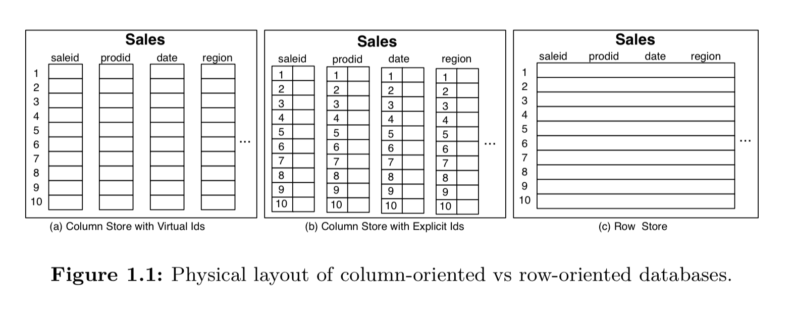
Data for a column may be stored in an array with implicit ids (a), or in some format with explicit ids (b).
Since data transfer costs from storage (or through a storage hierarchy) are often the major performance bottlenecks in database systems, while at the same time database schemas are becoming more and more complex with fat tables with hundreds of attributes being common, a column-store is likely to be much more efficient at executing queries… that touch only a subset of a table’s attributes.
Column stores are typically used in analytic applications, with queries that scan a large fraction of individual tables and compute aggregates or other statistics over them. (Whereas e.g. OLTP applications retrieving all attributes for a given row are better suited to row-based stores).
Making column stores fast
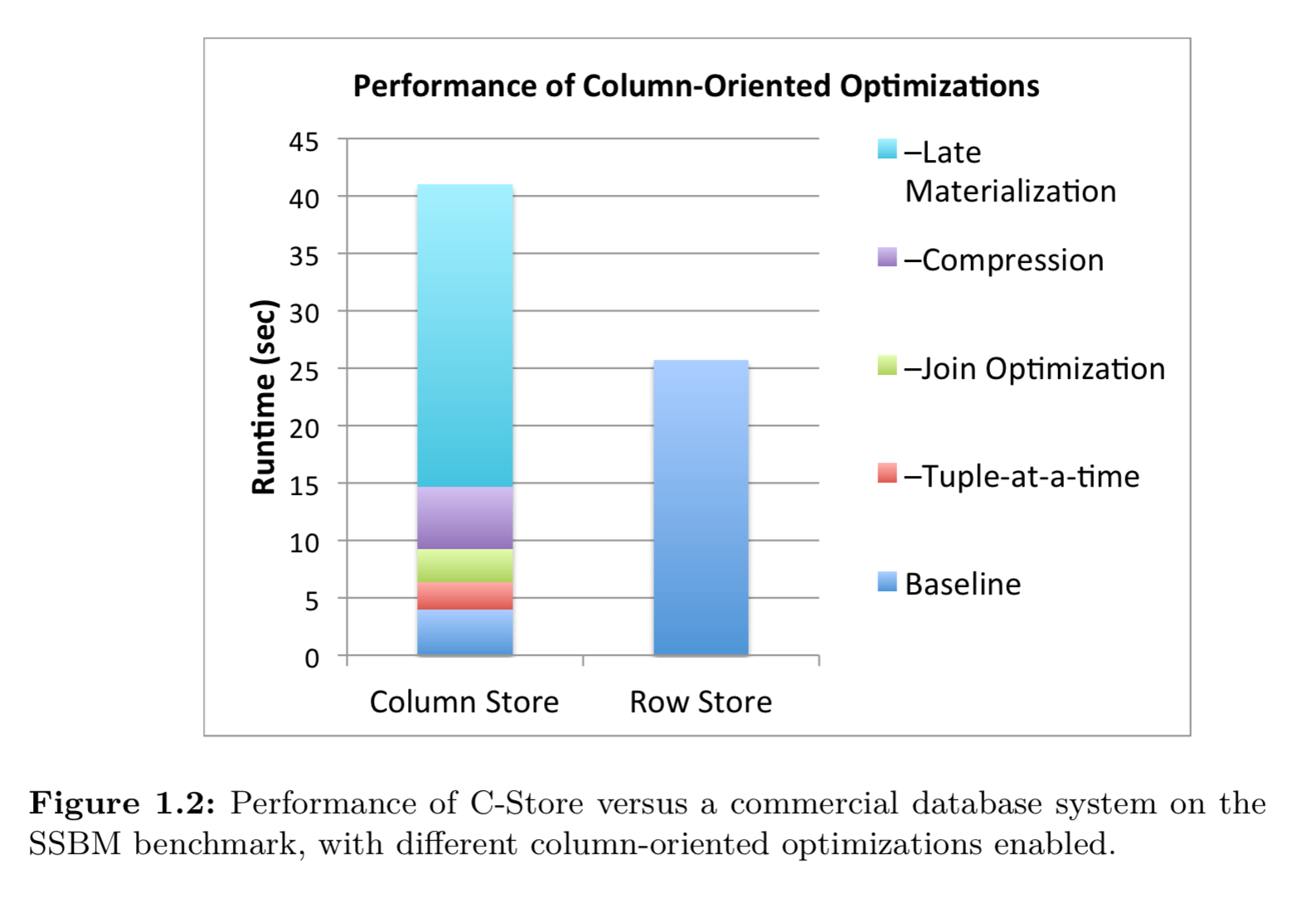
Simply storing data in columns isn’t sufficient to get the full performance out of column-based stores. There are a number of techniques that have been developed over the years that also make a big impact. The figure below shows an unoptimised column store performing worse than a row store on a simplified TPC-H benchmark. But by the time you add in a number of the optimisations we’re about to discuss, it ends up about 5x faster than the row store.
One of the most important factors in achieving good performance is preserving I/O bandwidth (by e.g. using sequential access wherever possible and avoiding random accesses). Thus even when we look at techniques such as compression, the main motivation is that moving compressed data uses less bandwidth (improving performance), not that the reduced sizes save on storage costs.
Pioneering column-store systems including MonetDB, VectorWise, and C-Store.
The following table summarizes some of the key techniques used in column-stores, and their row-store counterparts.
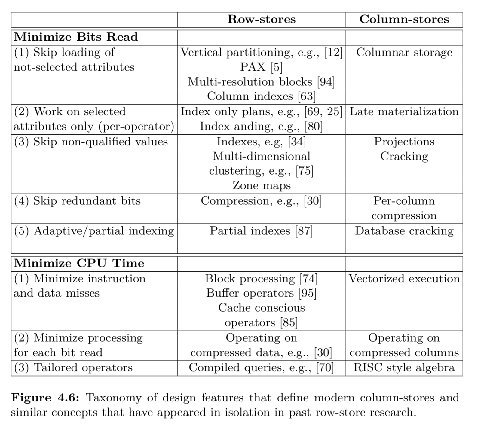
Let’s dive into some of these in more detail…
Block-oriented and vectorized processing
Traditional query execution uses a tuple-at-a-time pull-based iterator approach in which each operator gets the next input tuple by calling the next() method of the operators of its children in the operator tree.
MonetDB introduced the idea of performing simple operations one column at a time. To do this, it used lower level Binary Association Table (BAT) operators, with complex expressions in a query mapped into multiple BAT Algebra operations. “The philosophy behind the BAT Algebra can also be paraphrased as ‘the RISC approach to database query languages’.” VectorWise improved on MonetDB with a vectorised execution model striking a balance between the full materialization of intermediate results required by MonetDB and the high functional overhead of tuple-at-a-time iterators in traditional systems.
Essentially, VectorWise processes one block/vector of a column at a time as opposed to one column-at-a-time or one tuple-at-a-time.
The operators are similar to those used in tuple pipelining, excepte that the next() method returns a vector of N tuples instead of only one. Vectorised processing has a number of advantages including:
- Reduced function call overhead (N times fewer calls)
- Better cache locality with tuned vector sizes
- Opportunity for compiler optimisation and use of SIMD instructions
- Block-based algorithm optimisations
- Parallel memory access speed-ups through speculation
- Lower performance profiling overheads
- Better support for runtime adaptation based on performance profiling data.
Column-specific compression
Intuitively, data stored in columns is more compressible than data stored in rows. Compression algorithms perform better on data with low information entropy (i.e., with high data value locality), and values from the same column tend to have more value locality than values from different columns.
Compression improves performance by reducing the amount of time spent in I/O. With performance as a goal, CPU-light compression schemes are preferred. Different columns may of course use different compression schemes as appropriate.
Frequency partitioning makes compression schemes even more efficient by partitioning a column such that each page has as low an information entropy as possible (e.g., storing frequent values together).
Encoding schemes include:
- Run length encoding (RLE) which uses (value, start position, run length) triples.
- Bit-vector encoding, useful when columns have a limited number of possible data values. Each possible data value has an associated bit-vector, with the corresponding bit in the vector set to one if the column attribute at that position has the chosen value.
- Dictionary encodings (work well for distributions with a few very frequent values)
- Frame-of-reference encodings (save space by exploiting value-locality : values are represented by a delta from a base reference value).
With dictionary and frame-of-reference encodings patching may also be used. Here we encode only the most frequent values, and allow ‘exception’ values which are not compressed. Typically a disk block might be split into two parts that grow towards each other: compressed codes at the start of the block growing forwards, and an error array at the end growing backwards. For tuples with exception values, their encoded value is a special escape value signalling the value should be looked up separately.
Direct operation on compressed data
The ultimate performance boost from compression comes when operators can act directly on compressed values without needing to decompress. Consider a sum operator and RLE encoded values. It suffices to multiply the value by the run length.
To avoid lots of compression-technique specific code blocks the general properties of compression algorithms can be abstracted so that query operators can act on compression blocks.
A compression block contains a buffer of column data in compressed format and provides an API that allows the buffer to be accessed by query operators in several ways…
Compression alone can give up to a 3x performance improvement. By adding in operation on compressed data it is possible to obtain more than an order of magnitude in performance improvements.
Late materialization
Many queries access more than one attribute from a particular entity, and most database output standards (e.g. ODBC, JDBC) access results using an entity-at-a-time interface, not a column-at-a-time. Therefore at some point, a column store probably needs to re-assemble row-based tuples (‘tuple construction’).
The best performance comes from assembling these tuples as late as possible, operating directly on columns for as long as possible.
In order to do so, intermediate ‘position’ lists often need to be constructed in order to match up operations that have been performed on different columns.
The following figure illustrates a late materialization query plan for a select-project-join query. The select operators filter each column independently, maximising the utilisation of memory bandwidth.
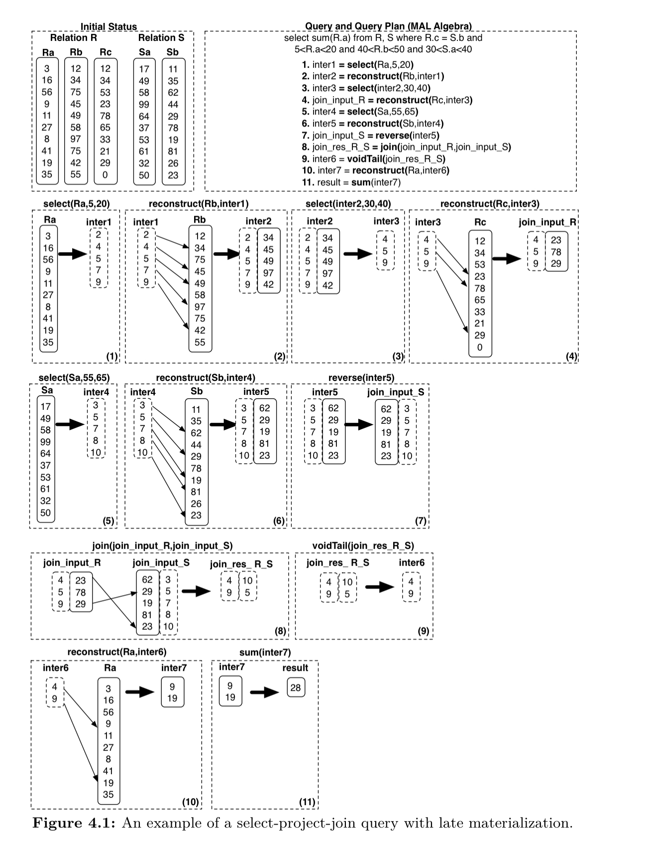
See section 4.4 in the paper for the full explanation of what’s going on here!
Late materialisation has four main advantages:
- Due to selection and aggregation operations, it may be possible to avoid materialising some tuples altogether
- It avoids decompression of data to reconstruct tuples, meaning we can still operate directly on compressed data where applicable
- It improves cache performance when operating directly on column data
- Vectorized optimisations have a higher impact on performance for fixed-length attributes. With columns, we can take advantage of this for any fixed-width columns. Once we move to row-based representation, any variable-width attribute in the row makes the whole tuple variable-width.
Efficient join implementations
The most straightforward way to implement a column-oriented join is for (only) the columns that compose the join predicate to be input to the join. In the case of hash joins (which is the typical join algorithm used) this results in much more compact hash tables which in turn results in much better access patterns during probing; a smaller hash table leads to less cache misses.
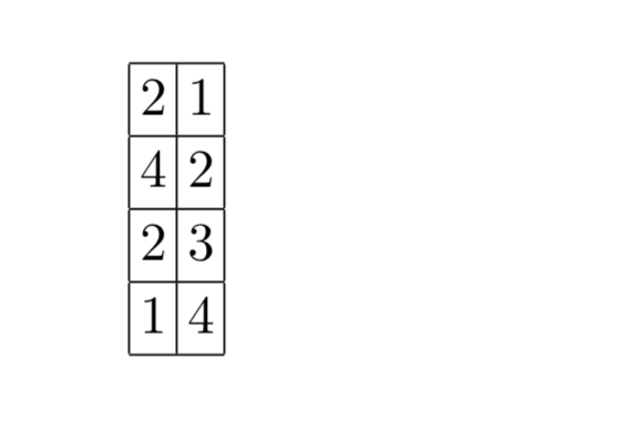
After a join, at least one set of output positions will not be sorted (e.g. the left input relation will have entries in sorted order, but the right output relation will not). That’s a pain when other columns from the joined tables are needed after the join. “Jive joins” add an additional column to the list of positions that we want to extract. Say we know we want to extract records 2, 4, 2, and 1 in that order. We add an ordering column thus:
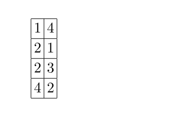
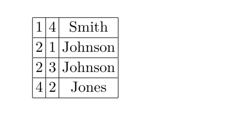
And then sort the output by the first column:
We can now scan the columns from the table efficiently to get the data.
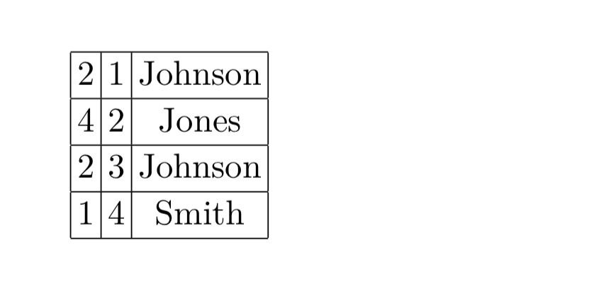
We sort by the second column (the ‘index’ that we added) to put the data back in the right order to complete the join.
Redundant column representations
Columns that are sorted according to a particular attribute can be filtered much more quickly on that attribute. By storing several copies of each column sorted by attributes heavily used in an application’s query workload, substantial performance gains can be achieved. C-store calls groups of columns sorted on a particular attribute projections.
Database cracking and adaptive indexing
An alternative to sorting columns up front is to adaptively and incrementally sort columns as a side effect of query processing. “Each query partially reorganizes the columns it touches to allow future queries to access data faster.” For example, if a query has a predicate A n where n ≥ 10, it only has to search and crack only the last part of the column. In the following example, query Q1 cuts the column in three pieces and then query Q2 further enhances the partitioning.
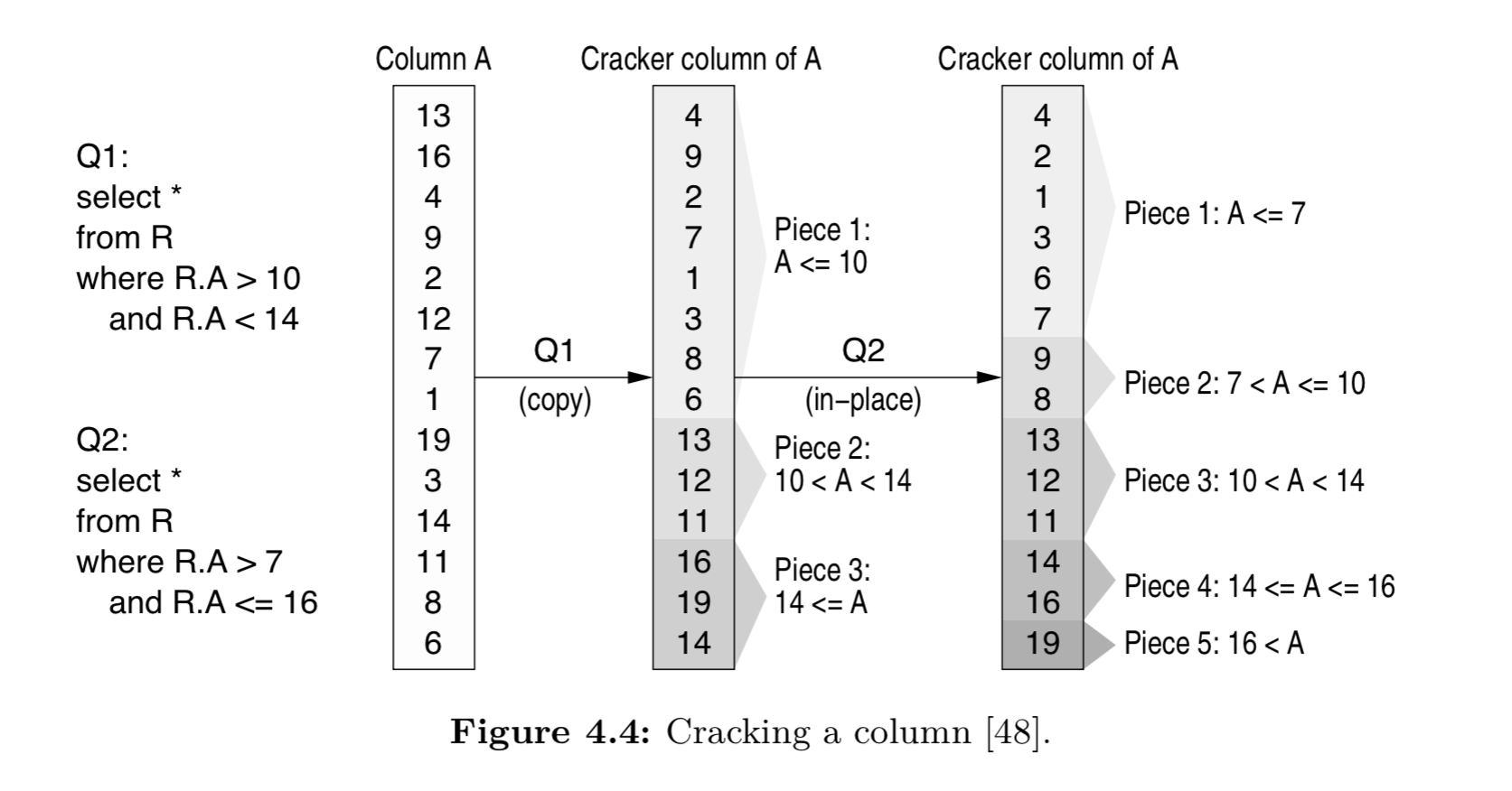
The terminology “cracking” reflects the fact that the database is partitioned (cracked) into smaller and manageable pieces.
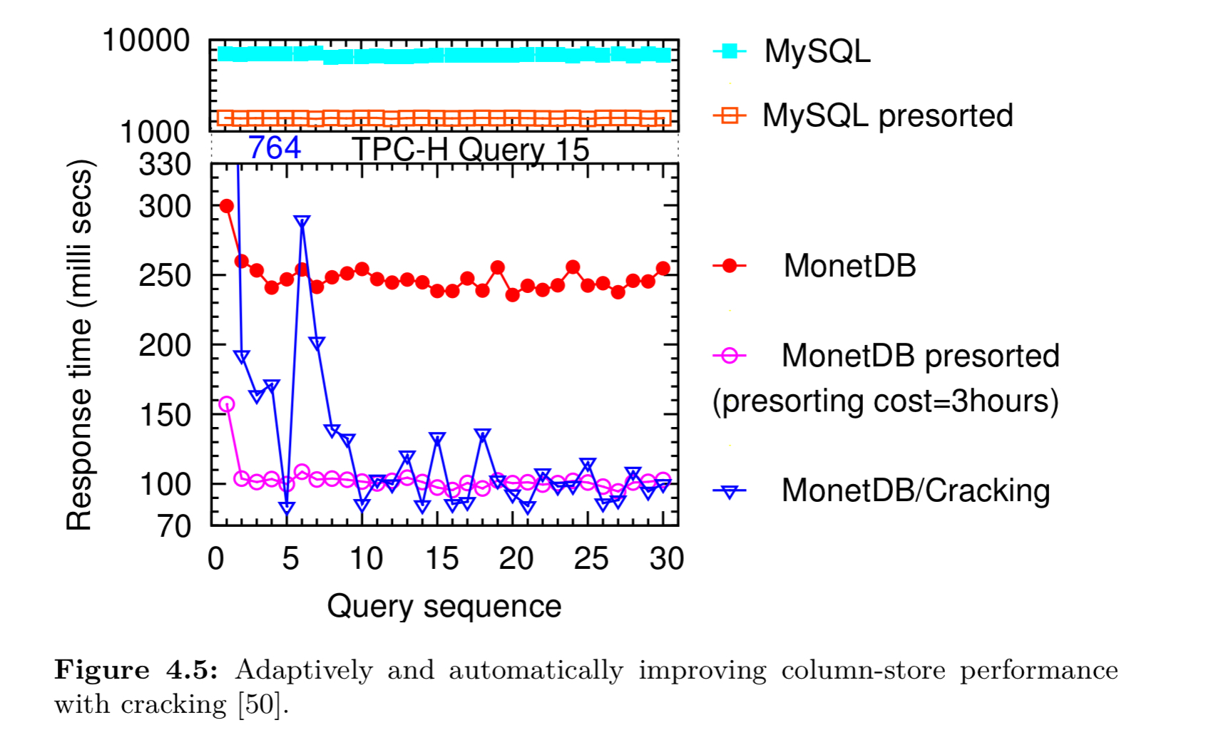
Cracking can bring big performance gains without paying the overhead of pre-sorting. Here’s an example from MonetDB:
A variation called stochastic cracking performs non-deterministic cracking actions by following query bounds less strictly. By doing so it can create a more even spread of the partitioning across a column.
Efficient loading
As a final thought, with all of this careful management of compressed columns going on you’d be right in thinking that updates (and deletes) are a pain. For analytic use cases, we generally want to load lots of data at once. The incoming data is row-based, and it needs to be split into columns with each column being written separately. Optimised loaders are important. The C-Store system for example first loads all data into an uncompressed write-optimised buffer, and then flushes periodically in large compressed batches.

Relevant to this, Apache Arrow: https://www.dremio.com/origin-history-of-apache-arrow/
Am I missing something, or does Figure 4.1 have a few errors? E.g. I think (3) select(inter2, 40, 50) and (5) should be select(Sa, 30, 40).
From what I can tell the descriptions are wrong on these, but the depicted selections are correct for given initial query.