Popular is cheaper: curtailing memory costs in interactive analytics engines Ghosh et al., EuroSys’18
(If you don’t have ACM Digital Library access, the paper can be accessed either by following the link above directly from The Morning Paper blog site).
We’re sticking with the optimisation of data analytics today, but at the other end of the spectrum to the work on smart arrays that we looked at yesterday. Getafix (extra points for the Asterix-inspired name, especially as it works with Yahoo!’s Druid cluster) is aimed at reducing the memory costs for large-scale in-memory data analytics, without degrading performance of course. It does this through an intelligent placement strategy that decides on replication level and data placement for data segments based on the changing popularity of those segments over time. Experiments with workloads from Yahoo!’s production Druid cluster that Getafix can reduce memory footprint by 1.45-2.15x while maintaining comparable average and tail latencies. If you translate that into a public cloud setting, and assuming a 100TB hot dataset size — a conservative estimate in the Yahoo! case — we’re looking at savings on the order of $10M per year.
Real-time analytics is projected to grow annually at a rate of 31%. Apart from stream processing engines, which have received much attention, real time analytics now includes the burgeoning area of interactive data analytics engines such as Druid, Redshift, Mesa, Presto, and Pinot.
Such systems typically require sub-second query response times. Yahoo!’s (Oath’s) Druid deployment has over 2000 hosts, stores petabytes of data, and serves millions of queries per day with sub-second latency. To get these response times, queries are served from memory.
Interactive data analytics
Data flows into an interactive data analytics engine via both batch and streaming pipelines. Data from streaming pipelines is collected by real-time nodes which chunk events by time interval and push them into deep storage. Such a chunk is called a segment. Segments are immutable units of data that can be placed on compute nodes (also known as historical nodes). One segment may be replicated across a number of nodes. A coordinator handles data management, creating and placing segment replicas. Clients send queries to a frontend router (broker), which maintains a map of which nodes are currently storing which segments. Queries often access multiple segments.
This paper proposes new intelligent schemes for placement of data segments in interactive analytics engines. The key idea is to exploit the strong evidence that an any given point in time, some data segments are more popular than others.
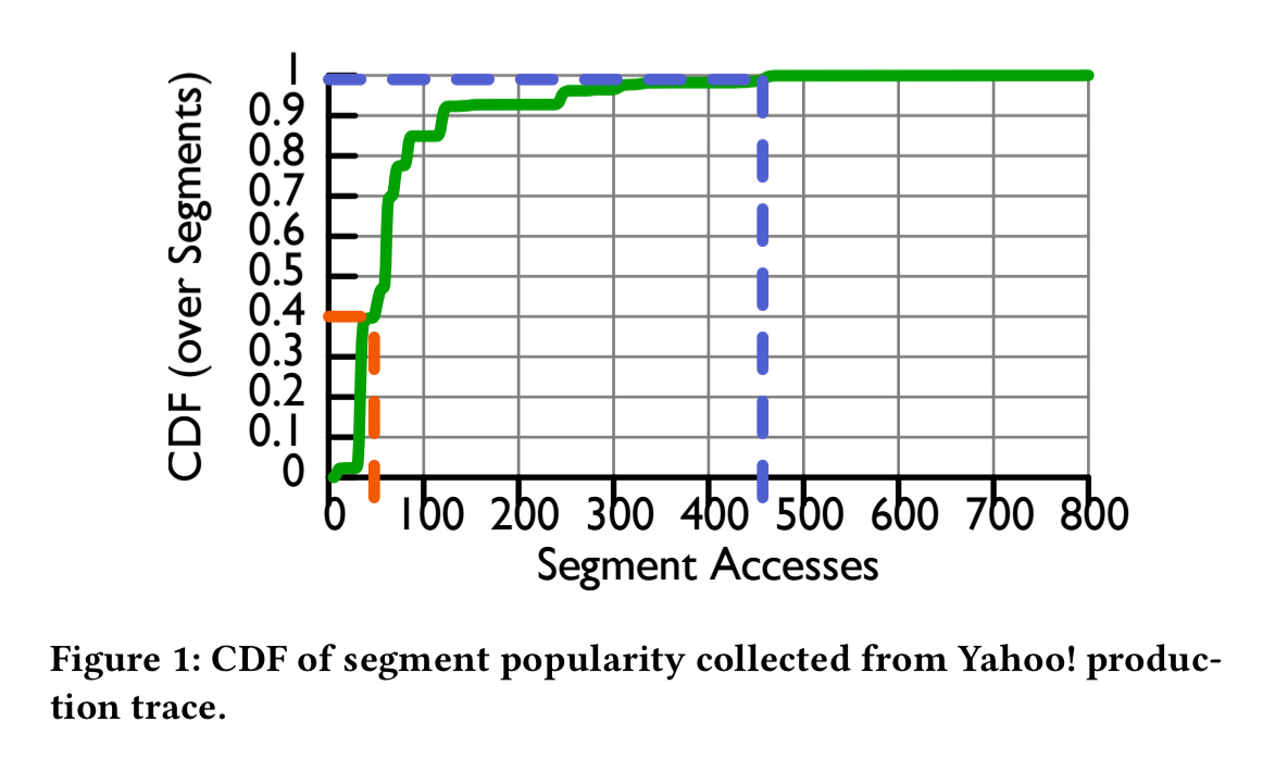
Let’s look at some of that evidence, based on Yahoo!s production Druid cluster workloads. Segment accesses show a clear skew, with more recent segments noticeably more popular than older ones. The top 1% of segments are accessed an order of magnitude more than the bottom 40% combined.
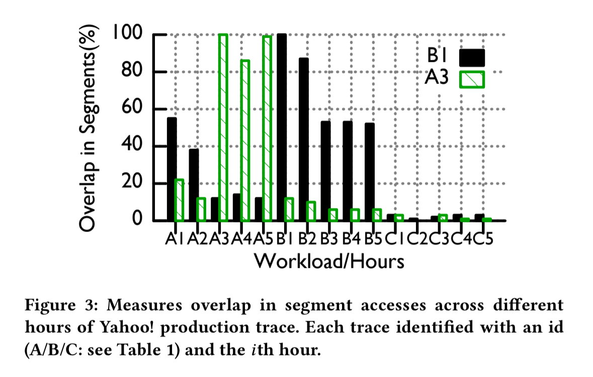
However, we can’t rely exclusively on recency. Some older segments continue to stay popular. The following figure shows the level of overlap between segments accessed during an hour of the Yahoo! trace and a reference hour (B1, A3). Traces labeled “A” are from October 2016, “B” traces are from January 2017, and “C” traces from February 2017. Segments from B1 have a 50% chance of co-occurring with segments from A1 that are five months older.
The average query latency for segments depends on the overall cluster size, the query rate, and the replication factor. In the following plot, the replication factor (on the x-axis) is the same for all segments, and the configurations are given as a (cluster size / query rate) pair. For example, the 15 / 2500 line is for a cluster with 15 historical nodes serving 2500 queries per second.
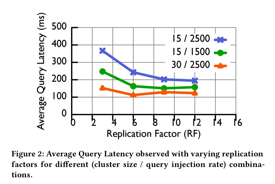
The thing to notice is that each line has a knee after which adding more replicas ceases to help (at 9 replicas for the 15/2500 configuration, and 6 replicas for the other two).
Our goal is to achieve the knee of the curve for individual segments (which is a function of their respective query loads), in an adaptive way.
Segments, balls, and bins
Let’s start with a static problem. Given n historical nodes, and k queries that access a subset of segments, how can we find a segment allocation that minimises both the total runtime and the total number of segment replicas? Assume for the moment that all queries take unit time per segment accessed, historical nodes have no segments loaded initially, and all historical nodes have equal compute power.
For each segment, count the number of distinct queries that access it. The example in the paper has 6 queries accessing four segments between them, with counts { S1:6, S2:3, S3:2, S4:1 } (i.e., segment one is accessed by all six queries, segment two by four of them, and so on). We can think of each query-segment pair as a coloured ball, with the the number of balls of that colour being the query count. A picture probably helps here:
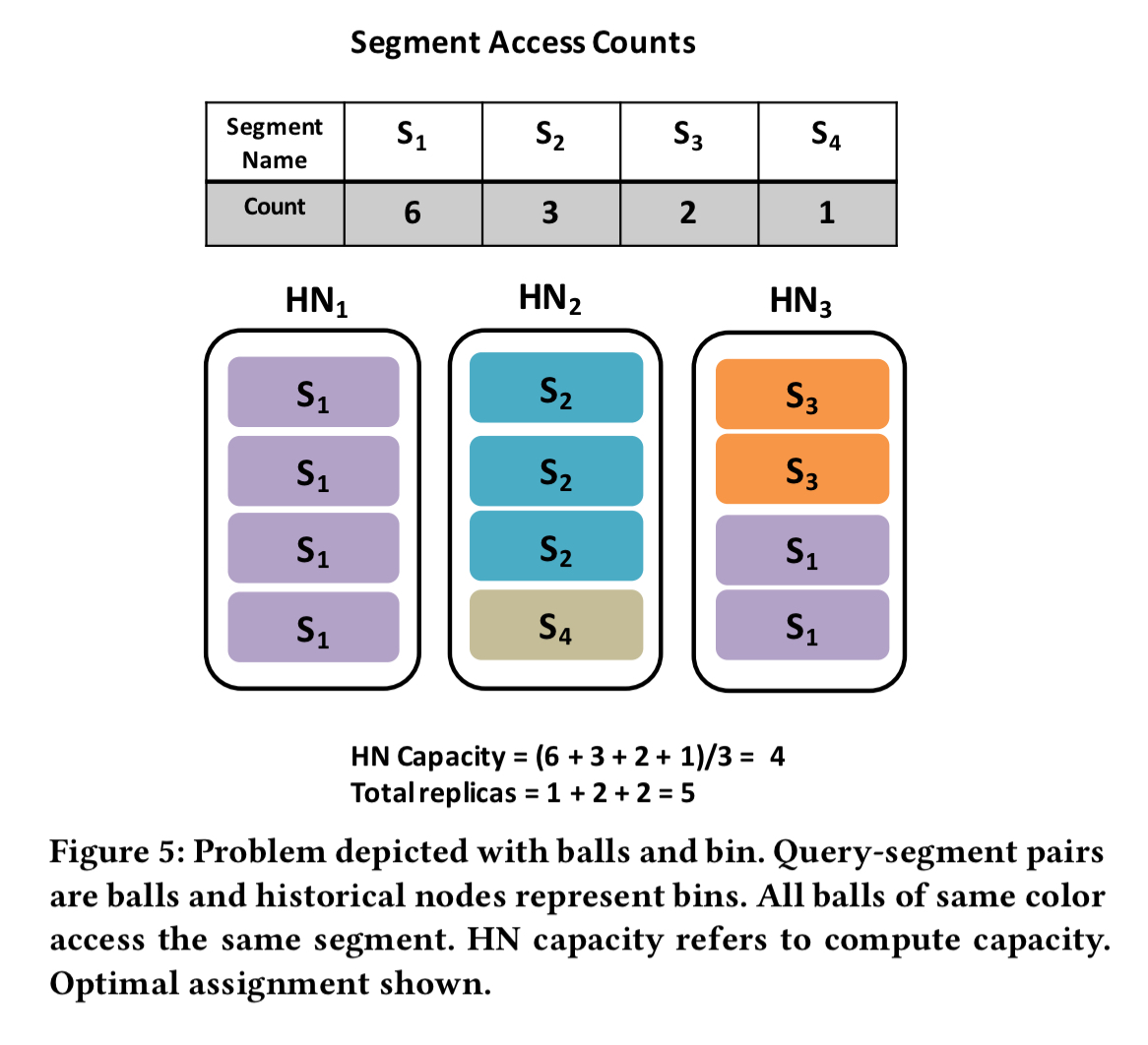
Let the historical nodes be bins, and we have a classic coloured-ball bin-packing problem.
The problem is then to place the balls in the bins in a load-balanced way that minimizes the number of “splits” for all colors, i.e., the number of bins each color is present in, summed up across all colors. The number of splits is the same as the total number of segment replicas. Unlike traditional bin packing which is NP-hard, this version of the problem is solvable in polynomial time.
Each coloured ball is a query access, so if each node has the same number of balls, each node will receive the same number of queries. So historical nodes will finish serving queries at the same time, giving the minimum total makespan. There are several ways we could put four balls in each node. To minimise the amount of memory required, we need to minimise the number of different colours at each node (i.e., the number of segments that node needs to keep in memory). This is what is achieved by minimising the number of splits.
The solution to the problem is given by algorithm 1 below:
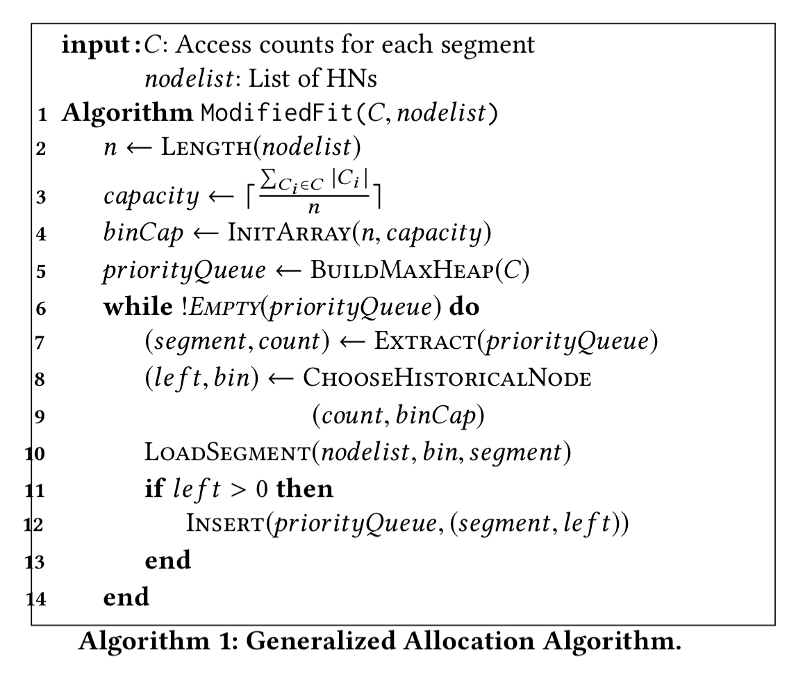
The algorithm maintains a priority queue of segments, sorted in decreasing order of popularity (i.e, number of queries accessing the segment). The algorithm works iteratively: in each iteration it extracts the next segment from the head of the queue, and allocates the query-segment pairs corresponding to that node to a historical node, selected based on a heuristic called ChooseHistoricalNode…
ChooseHistoricalNode works on a ‘best fit’ basis: it picks the node that has the least number of ball slots remaining after allocating all of the queries from the chosen segment to it. If no nodes have sufficient capacity, then the node with the largest available capacity is chosen. The leftovers, i.e., the unassigned queries (balls) are then put back into the sorted queue.
Extensions to the basic model
After each run of the algorithm above, a further balancing step takes place which looks to balance the number of segments (not balls) assigned to each node. This helps to minimise the maximum memory used by any historical node in the system. Let the segment load of a historical node be the number of segments assigned to it. Start with all the historical nodes that have higher than the above segment load. For those nodes, find the k least popular replicas on that node (where k is the difference between the given node’s segment load and the average). Add those replicas to a global re-assign list.
Now work through the list, and assign each replica to a historical node H such that:
- H does not already have a replica of the segment
- The query load imbalance after the re-assignment will be less than or equal to a configurable parameter γ (γ = 20% works well in practice). Query load imbalance is defined as 1 – (min query load for the node / max query load for the node).
- H has the least segment load of all historical nodes meeting criteria one and two.
If the cluster is not homogeneous, the algorithm can be further modified to distribute query load proportionally among nodes based on their estimate compute capacities. Node capacity is estimated by calculating the CPU time spent in processing queries. This approach has the nice side effect of automatically dealing with stragglers, which will tend to report lower CPU time in the sampling window (due to slow disk, flaky NIC, and other causes of waiting). The lesser reported capacity will then ensure popular segments are not assigned to these nodes.
Load balancing
Query routing decides which historical nodes hosting a replica of a segment a query should be routed to. Load based query routing was found to work the best. In this scheme, each broker keeps an estimate of every historical node’s current load (using the number of open connections it has to it as a proxy). An incoming query is routed to the historical node with the lowest load, out of those that host the desired segment.
Making it dynamic
Getafix handles dynamically arriving segments as well as queries. The overall system looks like this:
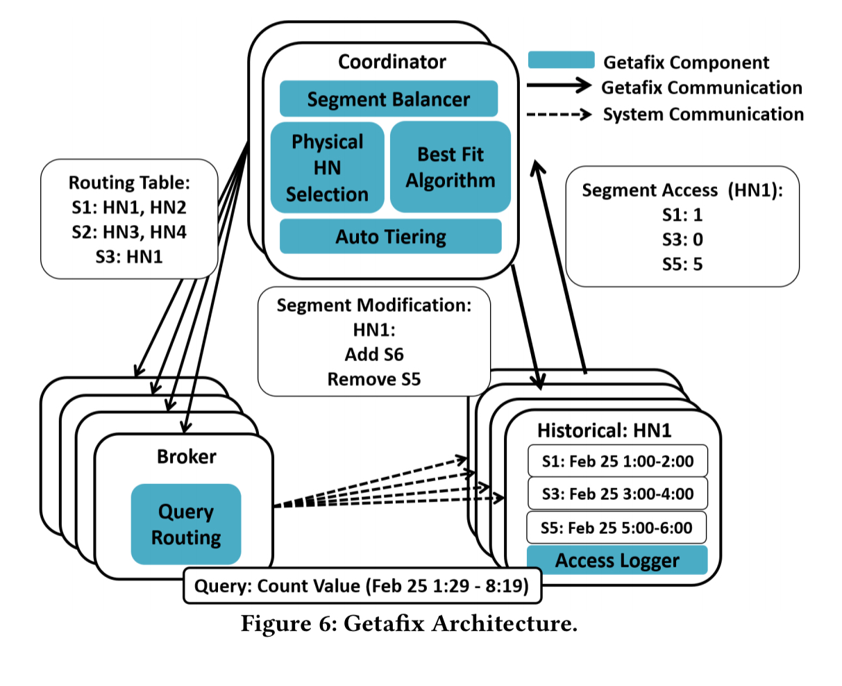
The static solution given above is run in periodic rounds. At the end of each round the query load statistics are gathered, the algorithm is run, and a segment placement plan produced. Then we can look at the delta between the new plan and the current configuration, and start moving things around. The coordinator calculates segment popularity via an exponentially weighted moving average, based on the total access time for each segment in each round. The current implementation sets the round duration to 5 seconds (seems very short to me!), “which allows us to catch popularity changes early, but not react too aggressively.”
Whereas today sysadmins typically manually configure clusters into tiers based on their hardware characteristics, Getafix’s capacity-aware solution essentially automatically discovers tiers, moving popular replicas to powerful historical nodes. This auto-tiering is unaware of network bandwidth constraints though.
There’s one more trick up the sleeve to try and minimise data movement. Consider the following scenario, with current HN assignments in the top row, and the assignments produced by the planner for the next round in the bottom row.
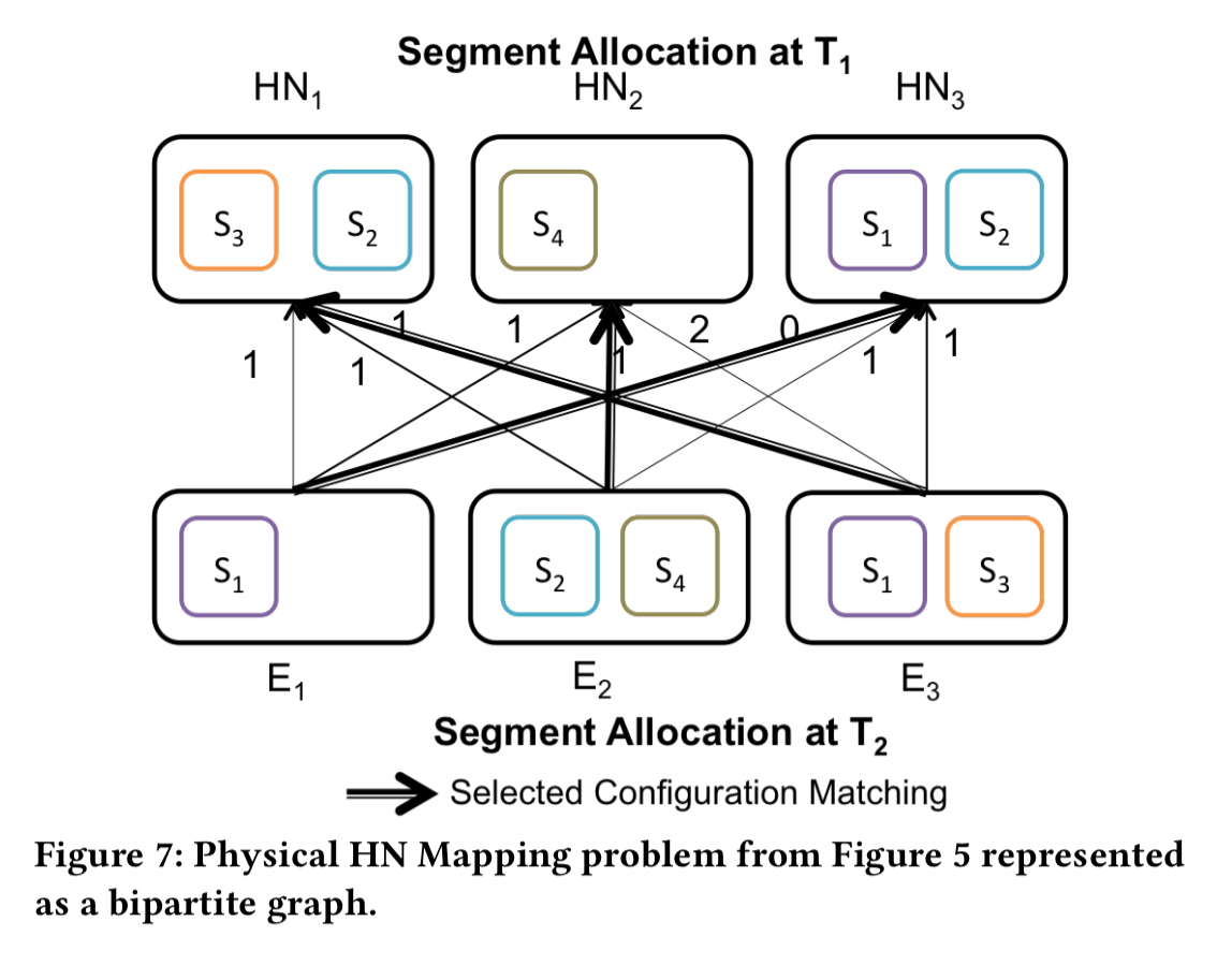
If do the straightforward thing, and make HN1 host the segments in E1, HN2 host the segments in E2, and HN3 host the segments in E3, we have to move 3 segments in total. But if instead we juggle the mapping of expected (E) packings to nodes such that E1 is mapped to HN3, E2 is mapped to HN2, and E3 is mapped to HN1 then we only have to move two segments. The Hungarian Algorithm is used to find the minimum matching. It has complexity 
Evaluation
I’m way over target length today trying to explain the core ideas of Getafix, so I’ll give just the briefest of highlights from the evaluation:
- Compared to the best existing strategy (from a system called Scarlett) Getafix uses 1.45-2.15x less memory, while minimally affecting makespan and query latency.
- Compared to the commonly used uniform replication strategy (as used by Druid today), Getafix improves average query latency by 44-55%, while using 4-10x less memory.
- The capacity-aware version of best fit improves tail query latency by 54% when 10% of nodes are slow, and by 17-22% when there is a mix of nodes in the cluster. In this case total memory is also reduced by 17-27%. A heterogeneous cluster is automatically tiered with an accuracy of 75%.
See section 5 in the paper for the full details!

Is it just me, or is anyone else confused by phrases like “Getafix can reduce memory footprint by 1.45-2.15x”? What does it mean to reduce something by 1.45 times? Might it be possible to rephrase this? (It reminds me of ads that promote home ‘smart-meters’ that say “reduce your energy bills by up to 100%”. Not as misleading as this, no doubt.)
@Zteve, Thanks for your comment. I would like to clarify the point. In our paper, we compare Getafix to another competing strategy Scarlett. In our experiments, we have observed that Getafix reduces memory usage by 1.45 – 2.15x compared to Scarlett.