Analytics with smart arrays: adaptive and efficient language-independent data Psaroudakis et al., EuroSys’18

(If you don’t have ACM Digital Library access, the paper can be accessed either by following the link above directly from The Morning Paper blog site).

We’re going lower-level today, with a look at some work on adaptive data structures by Oracle. It’s motivated by a desire to speed up big data analytic workloads that are “increasingly limited by simple bottlenecks within the machine.” The initial focus is on array processing, but the ambition is to extend the work to more data types in time.

Modern servers have multiple interconnected sockets of multi-core processors. Each socket has local memory, accessible via a cache-coherent non-uniform memory access (ccNUMA) architecture. In the NUMA world the following hold true:

• remote memory accesses are slower than local accesses
• bandwidth to a socket’s memory and interconnect can be separately saturated
• the bandwidth of an interconnect is often much lower than a socket’s local memory bandwidth

If we want to crunch through an array as fast as possible in a NUMA world, the optimum way of doing it depends on the details of the machine, and on the application access patterns. Consider a 2-socket NUMA machine, the figure below shows four possible arrangements:

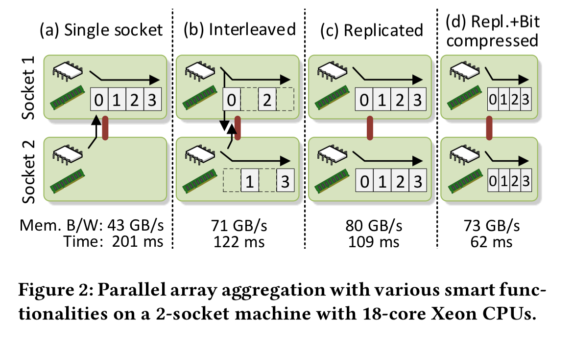
In (a) we place the array on a single socket, and access it from threads on both sockets. The bottleneck here will be the socket’s memory bandwidth. In (b) the array is interleaved across both sockets, and the bottleneck becomes the interconnect. In (c) the array is replicated, using more memory space but removing the interconnect as a bottleneck. In (d) the array’s contents are also compressed to reduce the memory usage resulting from replication. For this particular application, combination (d) is the fastest, but that won’t hold for all applications and all machines.

Smart arrays provide multiple implementations of the same array interface, so that trade-offs can be made between the use of different resources. In particular, they support multiple data placement options, in combination with bit compression. The selection of the best configuration can be automated. The selection algorithm takes as input:

1. A specification of the target machine, including the size of the memory, the maximum bandwidth between components, and the maximum compute available on each core.
2. The performance characteristics of the arrays, such as the costs of accessing a compressed item. This information is obtained from performance counters. It is specific to the array and the machine, but not the workload.
3. Information from hardware performance counters describing the memory, bandwidth, and processor utilisation of the workload.

Smart arrays can significantly decrease the memory space requirements of analytics workloads, and improve their performance by up to 4x. Smart arrays are the first step towards general smart collections with various smart functionalities that enable the consumption of hardware resources to be traded-off against one another.

Configuration options(aka ‘smart functionalities’)

There are four data placement options to choose from:

• OS default just uses the OS default placement policy. On Linux, this means physically allocating a virtual memory page on the socket on which the thread that first touches it is running.
• Single socket allocates the array’s memory pages on a specified socket
• Interleaved allocates the array’s memory pages across sockets in a round-robin fashion
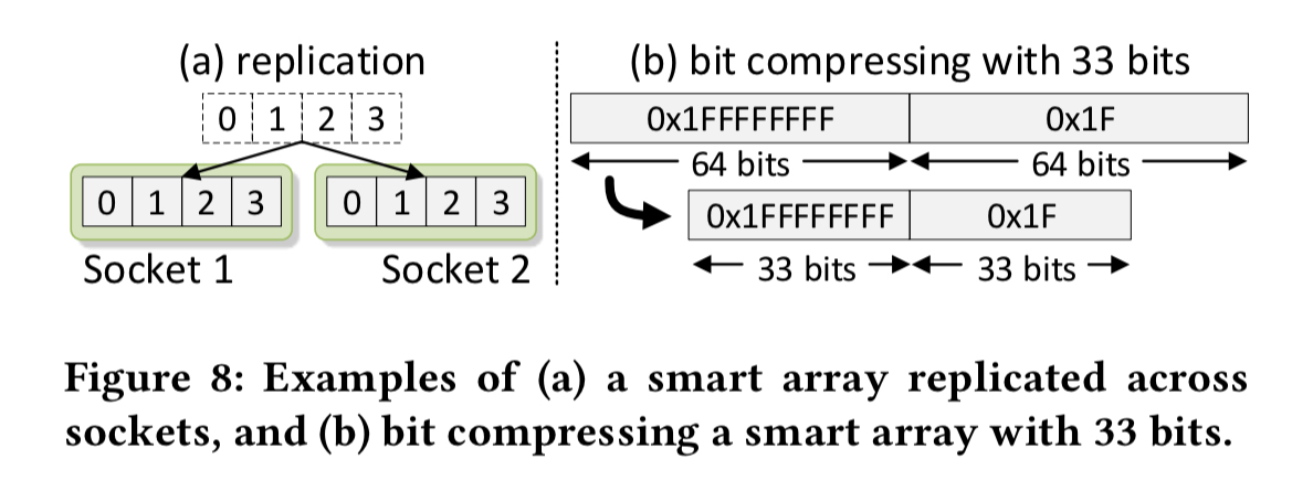
• Replicated places one replica of the array on each socket

In addition, we may opt to use bit compression for the array.

Bit compression is a light-weight compression technique that is popular for many analytics workloads such as column-store database systems. Bit compression uses less than 64 bits for storing integers that require fewer bits.

Bit compression increases the number of values per second that can be loaded through a given bandwidth. On the flip side, it increases the CPU instruction footprint. This can hurt performance compared to using uncompressed elements. However, if we’re hitting a memory bandwidth bottleneck, the compressed array can still be faster.

Assessing the impact of different configurations on a variety of workloads

We’ll briefly touch on implementation details later, but for now it suffices to know that Smart Arrays are implemented in C++ with efficient access from Java. Experiments are run with an aggregation workload, and a variety of graph analytics workloads.

The aggregation workload involves a parallel element-wise summation of two 4GB arrays of 64-bit integers. The experiment is conducted both from C++ and from Java, on an 8-core machine and on an 18-core machine. The results are shown in the following chart.

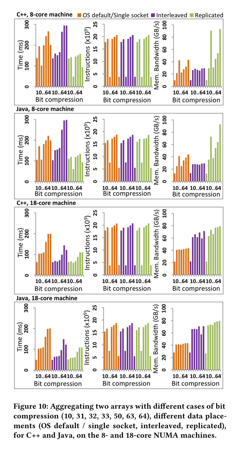
On the 8-core machine the interleaved placement is worst, since the limited bandwidth of the interconnect is less than a socket’s bandwidth. The single socket placement does better, exploiting the socket’s memory bandwidth, but the replicated placement is best of all, reducing the time by 2x.

The 18-core machine has much higher interconnect bandwidth. This is enough to make interleaving perform better than the single socket version, and replication only offers a slight advantage.

In this case, bit compression reduces the overall time by up to 4x compared to the OS default placement, or by up to 2x for the other data placements.

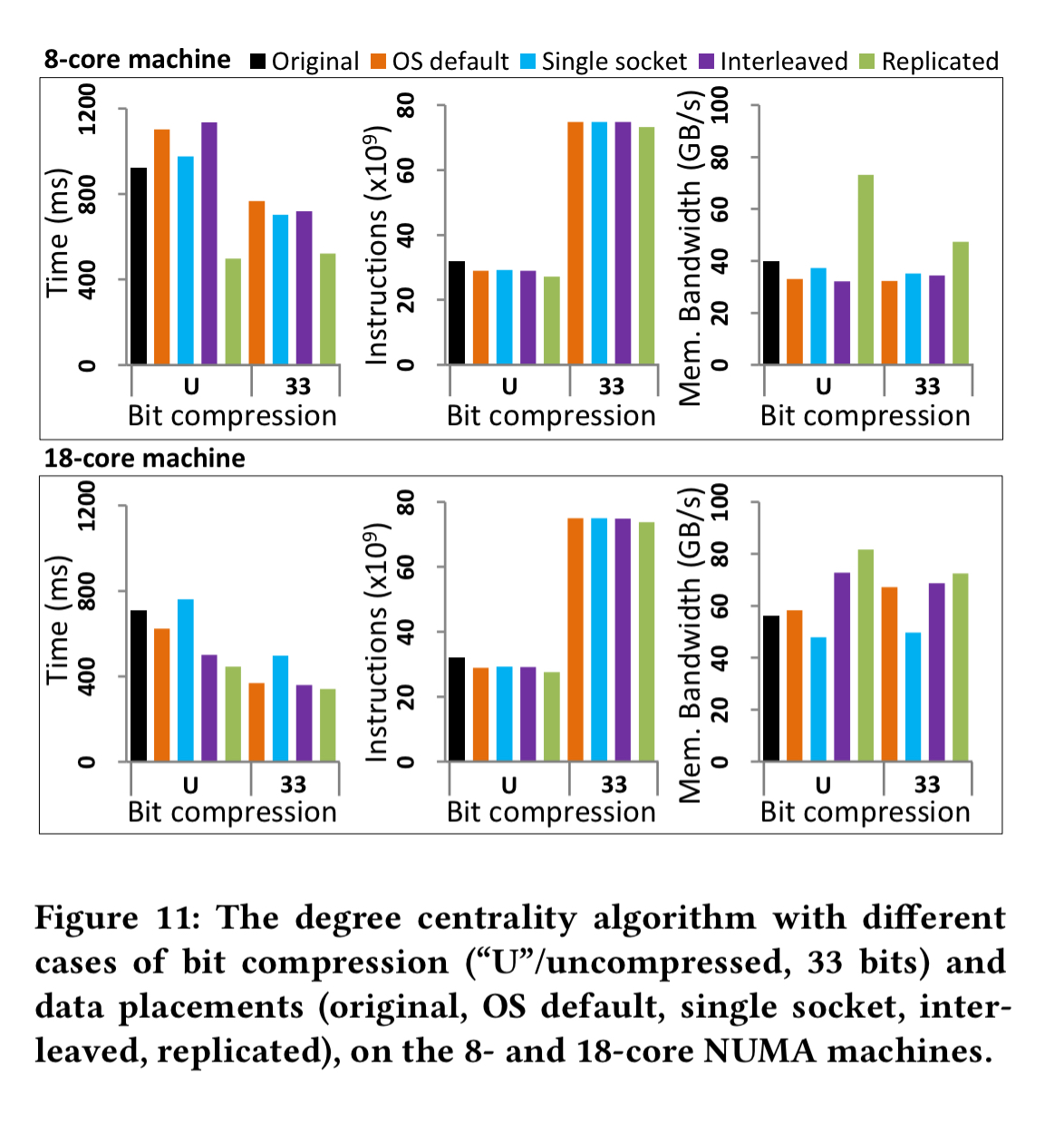
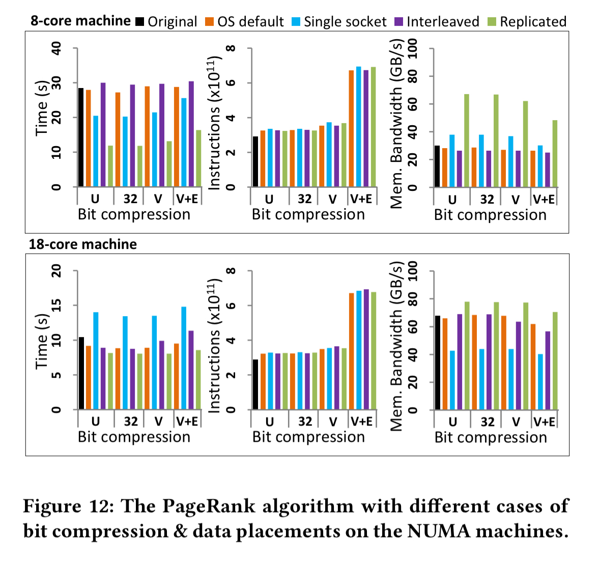
For graph analytics, a degree centrality computation and PageRank are used for the evaluation. With degree centrality on the 8 core machine replication again proves to be the best choice. The results are similar to the aggregation experiment for the 18-core case as well.

With PageRank replication on the 8-core machine gives up to a 2x improvement, but is not especially effective with 18 cores. Bit compression does not improve performance, but compressing both vertices and edges (V+E) can reduce memory space requirements by around 21%.

Automating the selection of the best configuration

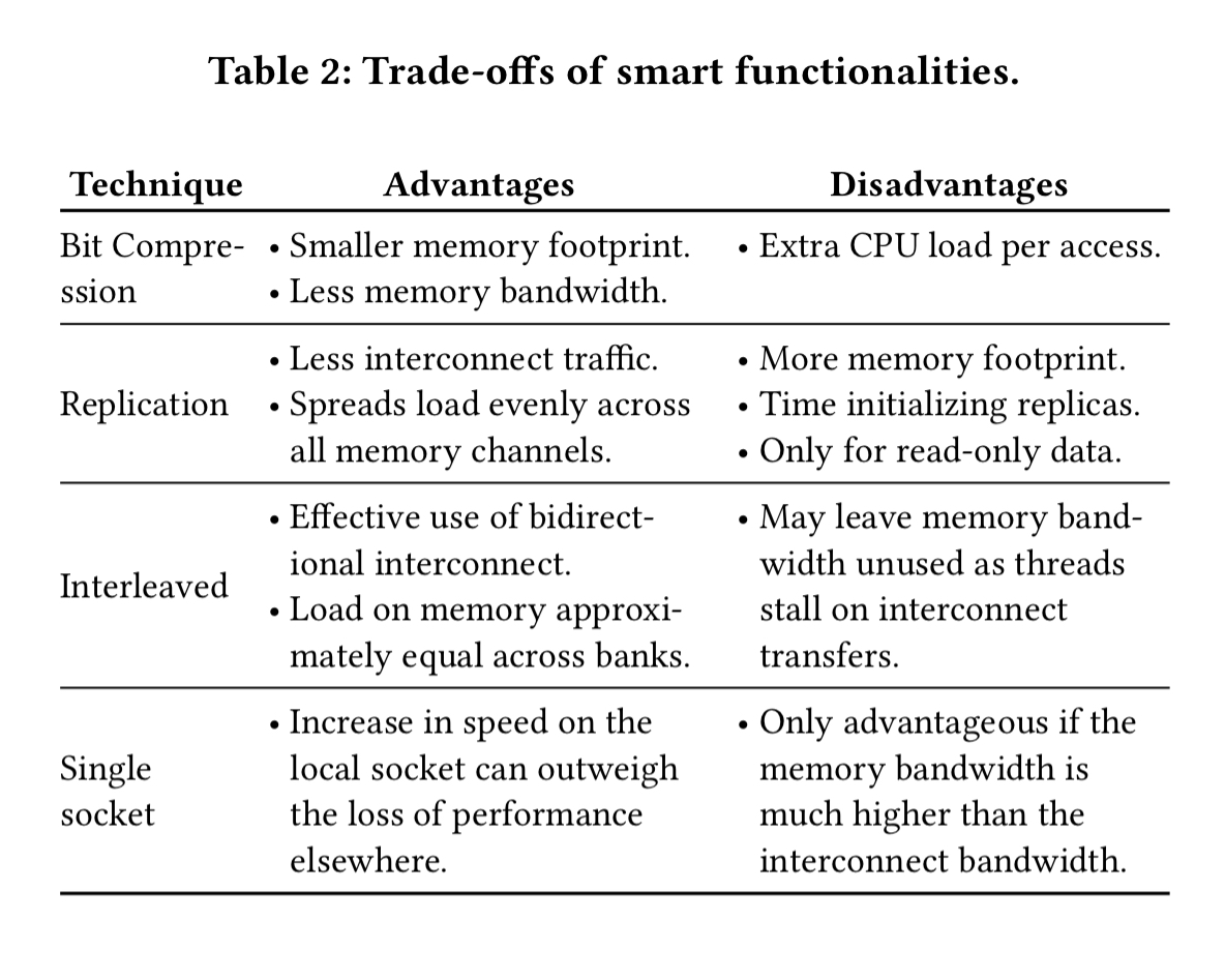
As we observe in the experimental evaluation, depending on the machine, the algorithm, and the input data, the cost, benefit, and availability of the optimisations can vary.

The following table summarise the trade-offs:

Rather than having to guess the best trade-offs by hand, the authors built an automated system for determining the best configuration, using the inputs we saw earlier in this post.

There are two decision flow charts, one to use when selection candidates without compression, and one to use when also including compression.

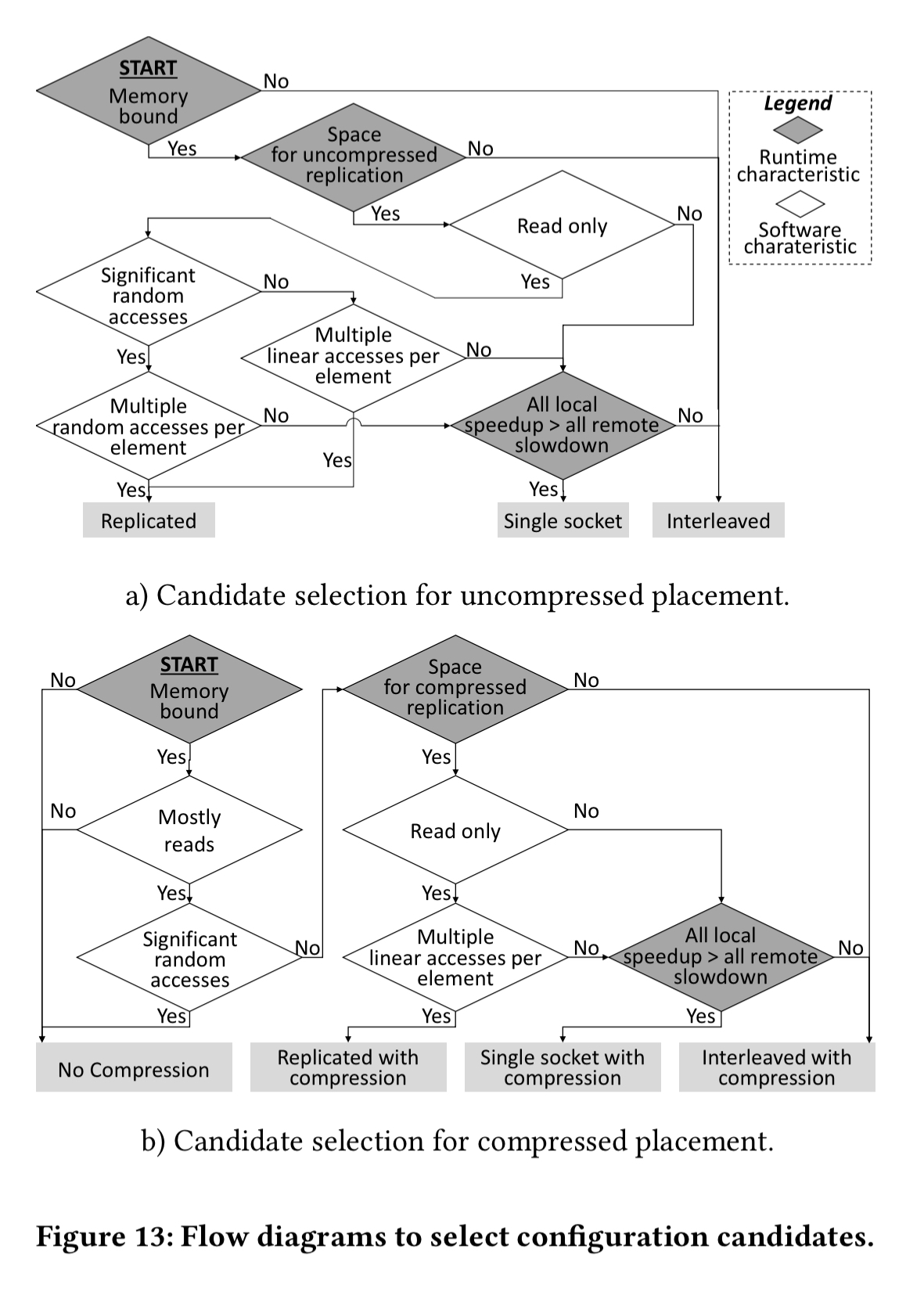
Following these decision charts, we will end up with two candidates: one with compression and one without. Now we have to decide which one of these two we should ultimately go with. We add back in to the compression profile estimate the additional compute required to perform compression based on the number of accesses per second and the cost per access. For each placement we compute two ratios per socked:

1. The ratio of the maximum compute rate relative to the current rate
2. The ratio of the maximum memory bandwidth for each candidate placement relative to the current bandwidth – this gives the socket speedup assuming the workload is not compute-bound.

The minimum of these two ratios is then taken as the estimated speedup of each socket, and the average across all sockets is taken as the estimated speedup given by the configuration. Pick the candidate configuration with the best estimated speedup!

The selection algorithm was evaluated using the aggregation and degree centrality workloads where the correct (best overall) placement was chosen 30 times out of 32.

The average performance of the selected configuration for each benchmark and hardware configuration paring was 0.2% worse than the optimal configuration for that pairing, and 11.7% better than then best static configuration.

Implementation details

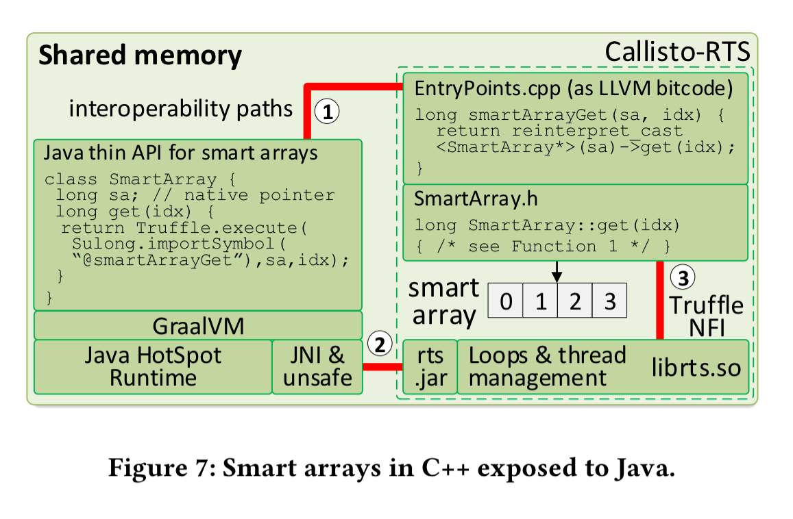
There’s quite a bit of detail in the paper, which I’ve skipped over entirely, concerning the C++ implementation and the way it is made efficiently accessible from Java. Here are the highlights:

• The implementation of the C++ library uses the Callisto runtime system, which supports parallel loops with dynamic distribution of loop iteration and includes a basic Java library to express loops.
• The GraalVM is used to create language-independent (Java and C++) smart arrays and use them efficiently from Java. The GraalVM (see ‘One VM to rule them all’) is a modified version of the Java HotSpot VM which adds Graal, a dynamic compiler implemented in Java, and Truffle, a framework for building high-performance language implementations.

The pieces all come together like this:

Future directions

• More data types including sets, bags, and maps. Smart arrays can be used to implement data layouts for these by encoding binary trees into arrays. It’s also possible to trade size against performance by using hashing instead of trees to index smart arrays.
• Additional smart functions including randomisation (fine-grained index-remapping of elements) to ensure that “hot” nearby data items are mapped to different locations. Also up for discussion are additional data placement techniques using domain specific knowledge, and alternative compression techniques which may achieve higher compression rates on some kinds of data.
• Runtime adaption, supporting runtime selection and re-selection of the best configuration based on the current workload.