Unsupervised anomaly detection via variational auto-encoder for seasonal KPIs in web applications Xu et al., WWW’18

(If you don’t have ACM Digital Library access, the paper can be accessed either by following the link above directly from The Morning Paper blog site, or from the WWW 2018 proceedings page).

Today’s paper examines the problem of anomaly detection for web application KPIs (e.g. page views, number of orders), studied in the context of a ‘top global Internet company’ which we can reasonably assume to be Alibaba.

Among all KPIs, the most (important?) ones are business-related KPIs, which are heavily influenced by user behaviour and schedule, thus roughly have seasonal patterns occurring at regular intervals (e.g., daily and/or weekly). However, anomaly detection for these seasonal KPIs with various patterns and data quality has been a great challenge, especially without labels.

Donut is an unsupervised anomaly detection algorithm based on Variational Auto-Encoding (VAE). It uses three techniques (modified ELBO, missing data injection, and MCMC imputation), which together add up to state-of-the-art anomaly detection performance. One of the interesting findings in the research is that it is important to train on both normal data and abnormal data, contrary to common intuition.

The problem

We’re interested in time series KPIs influenced by user behaviour and schedules, and thus have seasonal patterns (e.g. daily and/or weekly patterns). The precise shapes of the KPI curves in each cycle are not exactly the same of course, since user behaviour can vary across days.

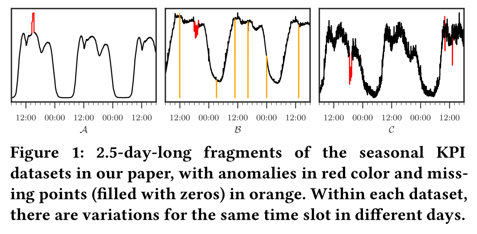
We also assume some (Gaussian) noise in the measurements. Anomalies are recorded points that do not follow normal patterns (e.g. spikes or dips). In additional to anomalies, there may also be missing data points where the monitoring system has not received any data. These points are recorded as ‘null’. Missing data points are not treated as anomalies.

We want to give a real valued score for each data point, indicating the probability that it is anomalous. A threshold can then be used to flag anomalies.

As part of the training set, we also have occasional labels where e.g. operators have annotated points. The coverage of these labels is far from what’s needed for typical supervised learning algorithms.

We aim at an unsupervised anomaly detection algorithm based on deep generative models with a solid theoretical explanation, that can take advantage of the occasionally available labels.

Deep generative models, VAEs, and Donut

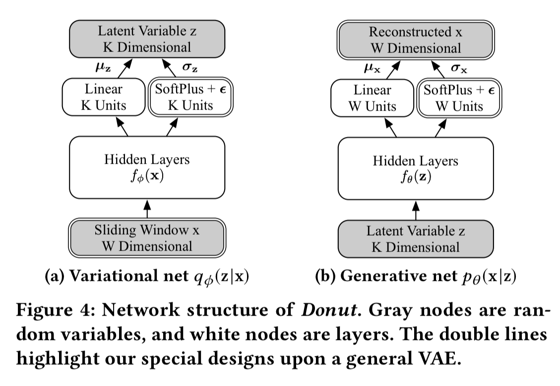
Learning what normal looks like — i.e., learning the distribution of training data — is something that generative models are good at. Variational Auto-Encoders provide a good starting point, but they’re not designed for sequence-based input. A simple solution here is to use sliding windows over the time series to create the input vector. With a window of size W, the input for a point will be .

This sliding window was first adopted because of its simplicity, but it turns out to actually bring an important and beneficial consequence…

The network structure of Donut looks like this:

M-ELBO

Training the VAE involves optimising the variational lower bound, aka. the evidence lower bound or ELBO. Since we want to learn normal patterns, we need to avoid learning abnormal patterns wherever possible. Both anomalies and missing values in the training data can mess this up. (Of course, we only know we have an anomaly if it is one of the occasional labeled ones available to us, unlabelled anomalies cannot be accounted for in this step).

One might be tempted to replace labeled anomalies (if any) and missing points (known) in training data with synthetic values… but it is hard to produce data that follow the ‘normal patterns’ well enough. More importantly, training a generative model with data generated by another algorithm is quite absurd, since one major application of generative models is exactly to generate data!

Instead, all missing points and labelled anomalies are excluded from the ELBO calculation, with a scaling factor to account for the possibly reduced number of points considered. This is the Modified-ELBO (M-ELBO) loss function (see Eqn. 3 in the paper).

Missing data injection

Not content with points that are naturally missing, a proportion of normal points are deliberately set to zero as if they were missing.

With more missing points, Donut is trained more often to reconstruct normal points when given abnormal , thus the effect of M-ELBO is amplified.

MCMC imputation

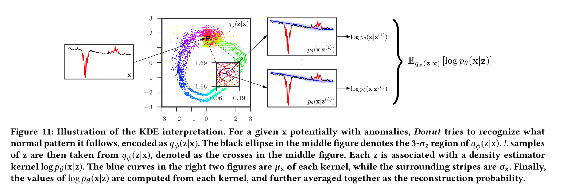
When we’re using the model to detect anomalies, we want to know how likely an observation window is, which we can estimate by considering its reconstruction probability. If there are missing values in the input though, that’s going to mess things up for us. So during anomaly detection, missing values in the input window are replaced using data imputation (i.e., by guessing what the recorded values would have been, had we captured them). This is done using the MCMC-based missing data imputation technique proposed by Rezende et al.

The input is split into observed () and missing () parts. Now we take the (whole) input and run it through the encoder to get a sample, and run that sample through the decoder to get a reconstruction . Throw away the first part of this reconstruction, but keep the reconstruction of the missing part, to produce a new input pair . Repeat this process M times, and use the final value of to fill in the missing data.

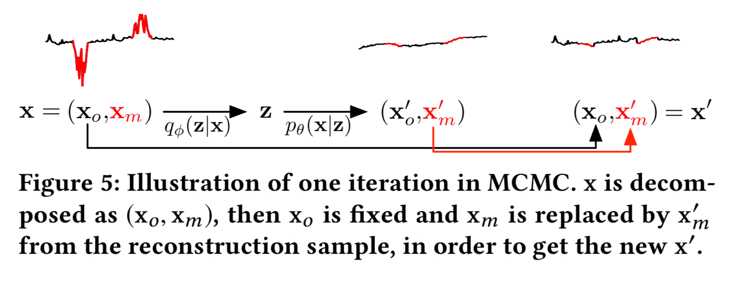
After this process, L samples are taken from to compute the reconstruction probability by Monte Carlo integration.

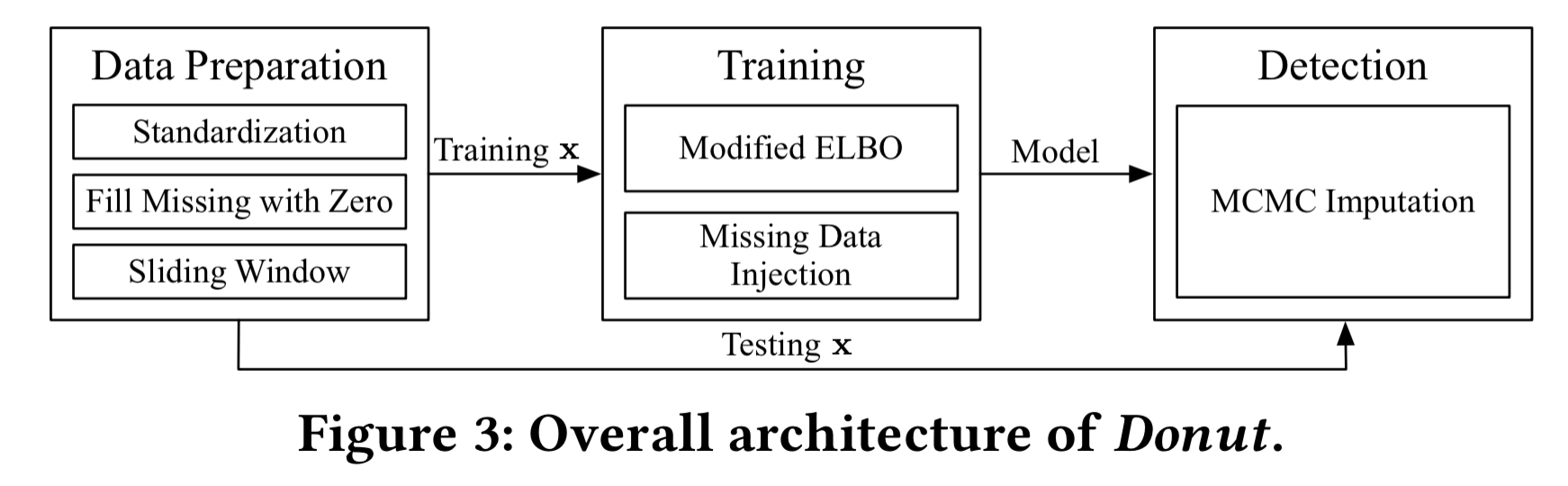
Putting it all together, the overall Donut process looks like this:

Evaluation

We can see the contribution of the three techniques above, which compares a VAE baseline to Donut with various combinations of them. A, B, and C are three different KPI series from our ‘top global Internet company.’

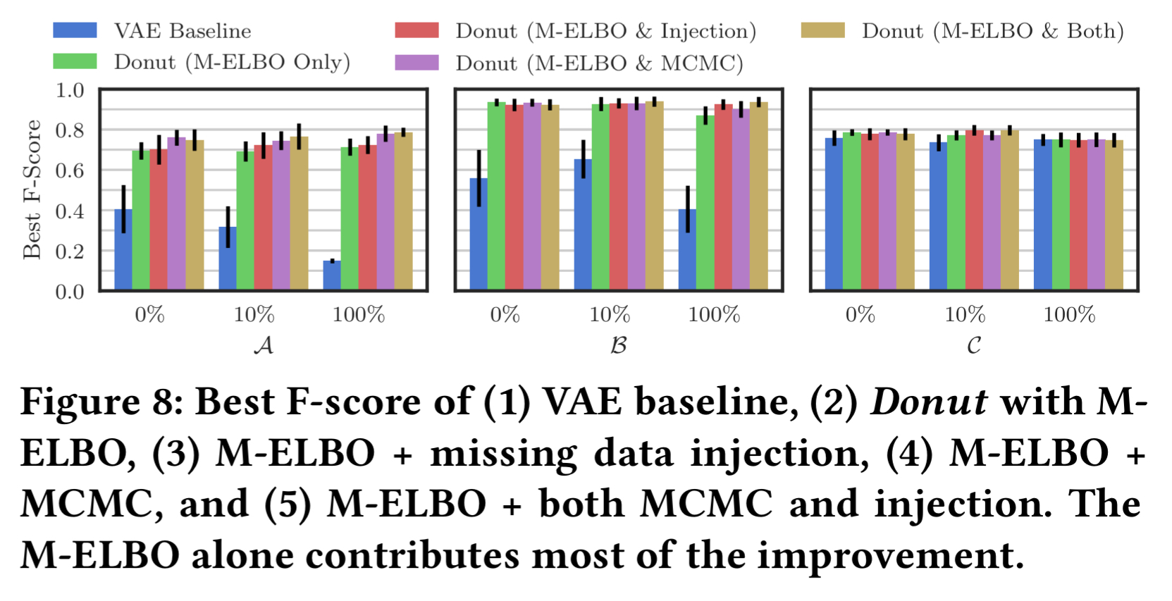
M-ELBO has the biggest impact.

[M-ELBO] works by training Donut to get used to possible abnormal points in , and to produce desired outputs in such cases. Although we expected M-ELBO to work, we did not expect it to work so well. In conclusion, it would not be a good practice to train a VAE for anomaly detection using only normal data, although it seems natural for a generative model. To the best of our knowledge, M-ELBO and its importance has never been stated in previous work, and thus is a major contribution of ours.

Missing data injection doesn’t show much additional improvement in the test, but this in counterbalanced by the fact that the extra randomness introduced to training should demand longer training times. Being unsure how much longer to train for to give a fair comparison, the authors used the same number of epochs across all configurations in the test. “We still recommend to use missing data injection, even with a cost of larger training epochs, as it is expected to work with a large chance.” It would have been nice to have seen a separate experiment to prove this, rather than just have to take it on faith.

MCMC imputation gives significant improvement in some cases, in other cases not so much. But since it never harms performance the recommendation is to always adopt it.

Interpretation: why does it work so well?

Section 5 contains an interpretation of what Donut is doing behind the scenes, “making it the first VAE-based anomaly detection algorithm with a solid theoretical explanation.” I find this part of the paper pretty hard going, but at a minimum I think I figured out where the name comes from!

If you set K=2 such that after the encoding we have z-variables with two dimensions, and then plot these on a chart you get a donut shape, as shown in (a) below.

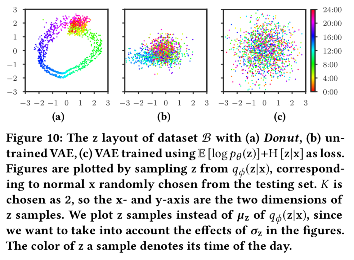
The colours of the points in the chart are an overlay representing the time of day of the sample. What we see is that points close in time in the original series are mapped close together in the z-space, causing the smooth colour gradient. The authors call this the ‘time gradient’. Strictly though, it’s not caused by wall-clock or even relative time, since time does not feature as an input. Instead, it’s caused by the transitions in the shape of over time.

The dimension reduction causes Donut to be able to capture only a small amount of information from , so only the overall shape can be encoded. Abnormal information is likely to be dropped in this procedure. The reconstruction probability in Donut can be viewed as a density estimator, indicating how well the input is following the learned . This gives rise to an interpretation of Donut as carrying out weighted kernel density estimation (KDE).

(Enlarge)