Equality of opportunity in supervised learning Hardt et al., NIPS’16

With thanks to Rob Harrop for highlighting this paper to me.

There is a a lot of concern about discrimination and bias entering our machine learning models. Today’s paper choice introduces two notions of fairness: equalised odds, and equalised opportunity, and shows how to construct predictors that are fair under these criteria. One very appealing feature of the model is that in the case of uncertainty caused by under-representation in the training data, the cost of less accurate decision making in that demographic is moved from the protected class (who might otherwise for example not be offered loans), to the decision maker. I’m going to approach the paper backwards, and start with the case study, as I find a motivating example really helps with the intuition.

Loans, race, and FICO scores

We examine various fairness measures in the context of FICO scores with the protected attribute of race. FICO scores are a proprietary classifier widely used in the United States to predict credit worthiness. Our FICO data is based on a sample of 301,536 TransUnion TransRisk scores from 2003.

We’re interesting in comparing scores, the risk of defaulting on a loan, and race. In the dataset, race is restricted to four values: Asian, white non-Hispanic (labeled ‘white’ in figures), Hispanic, and black. The scores are the results of complicated proprietary classifiers. But are they fair? And how should we think about fairness? A threshold score of 620 is commonly used for prime-rate loans, and that corresponds to an any account default rate of 18% (that is, 82% do not default).

Here are the marginal distributions for each group:

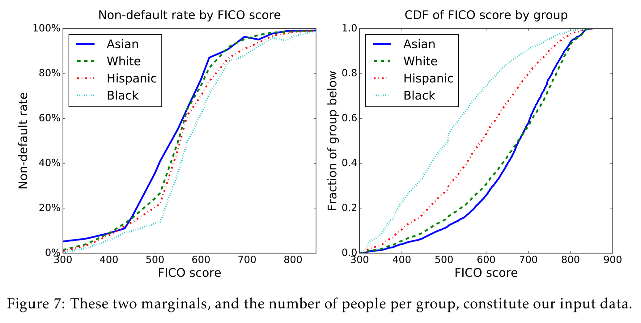
A max profit model with no fairness constraints at all picks a different threshold for each group, such that 82% of the people in that group do not default. It’s easy to see for example that this makes it less likely for a black person to get a loan than for an Asian person.

Next we might try a race blind model. This model requires the threshold to be the same for every group, so it picks a single threshold at which 82% of people do not default overall. Such a model would extract 99.3% of the profit available under the max profit model. This sounds good on the surface, but when you dig into it and examine per-group what it means to reach that single cut-off, it becomes readily apparent that it is not actually “fair” and disadvantages blacks and Hispanics vs whites and Asians:

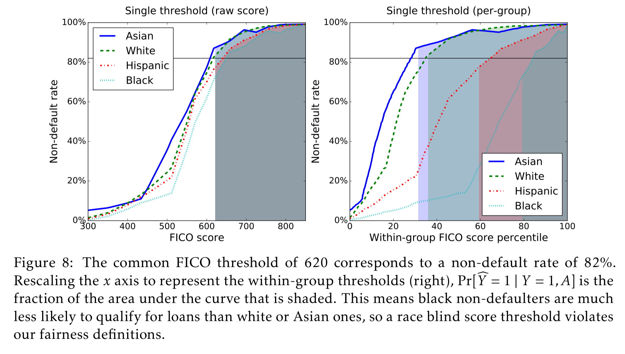
When race is redundantly encoded (i.e., it can be inferred from other variables), then race blindness degenerates into max profit.

Moving on, a popular approach to fixing the issues with the race blind is demographic parity. Under demographic parity we go back to choosing a different threshold for each group, but instead of choosing that threshold based on likelihood of default, we choose it such that the fraction of group members that qualify for loans is the same across all groups. That sounds good initially too…

Unfortunately, as was already argued by Dwork et al., the notion (of demographic parity) is seriously flawed on two counts. First, it doesn’t ensure fairness. Indeed, the notion permits that we accept qualified applications in the demographic A = 0, but unqualified individuals in A = 1, so long as the percentages of acceptance match. This behaviour can arise naturally when there is little or no training data available within A = 1. Second, demographic parity often cripples the utility that we hope to achieve.

(In the above paragraph, it’s assumed that the attribute A takes on a binary value, but it’s easy to generalise to the categorical case).

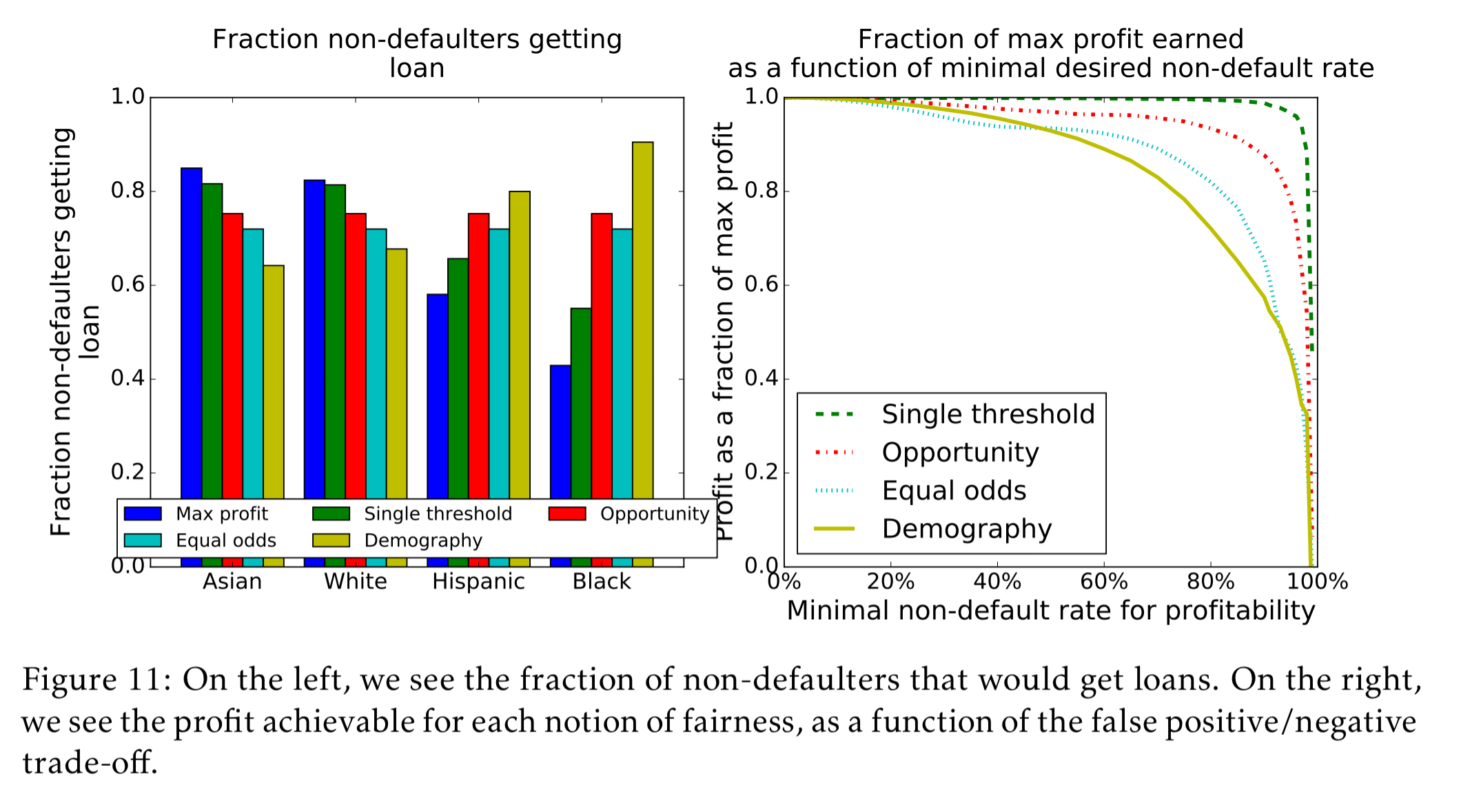
In the FICO dataset we’re looking at, using demographic parity obtains only 69.8% of profit available under the max profit model, and actually ends up reversing the bias such that e.g. white people that would not default have a significantly harder time qualifying for loans.

So now we arrive at the first of the two models introduced in the paper, equal opportunity. Equal opportunity requires non-discrimination only within the ‘advantaged’ outcome group. In this case, it says that people who pay back their loan, have an equal opportunity of getting the loan in the first place. For people that will end up defaulting, we do not require equal opportunity of getting a loan in the first place. To achieve equal opportunity, we pick per-group thresholds such that the fraction of non-defaulting group members that qualify for loans is the same across all groups. Equal opportunity does much better than demographic parity, extracting 92.8% of the potential profit available under the max profit model.

Even stronger than equal opportunity is equalized odds.

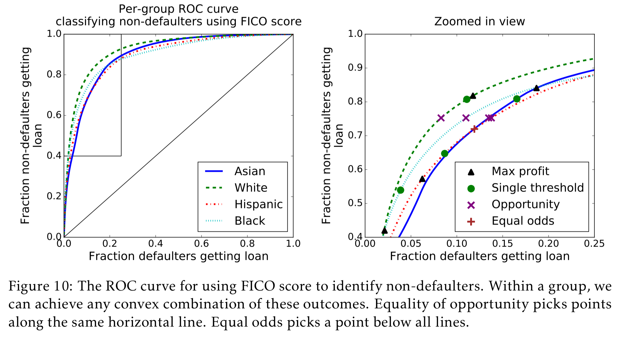
Equalized odds requires both the fraction of non-defaulters that qualify for loans and the fraction of defaulters that qualify for loans to be constant across groups. This cannot be achieved with a single threshold for each group, but requires randomization. There are many ways to do it; here we pick two thresholds for each group, so above both thresholds people always qualify, and between the thresholds people qualify with some probability.

Equalized odds achieves 80.2% of the potential profits available under the max profits model. The difference comes down to the fact that under equal opportunity the classifier can make use of its better accuracy among whites, but under equal odds this is viewed as unfair, since white people who wouldn’t pay their loans have a harder time getting them than minorities who wouldn’t pay their loans. “An equal odds classifier must classify everyone as poorly as the hardest group, which is why it costs over twice as much in this case.”

The following charts show visually the performance of the five different models discussed so far in terms of the fraction of non-defaulters that can successfully obtain loans, and the fraction of the maximum profit that is achieved.

You can also see how the FICO score thresholds vary across models:

Formalising equal odds and equal opportunity

Let X be the set of available features as input to a model, and A be the protected attribute (e.g., race in the example above). Y is the true outcome (i.e., the labels in our labeled dataset), is the predictor which predicts a value of Y given X. We’ll start with the case where Y is a binary decision and A is a binary attribute.

The notion we propose is “oblivious,” in that it is based only on the joint distribution, or joint statistics, of the true target Y, the predictions , and the protected attribute A. In particular, it does not evaluate the features in X nor the functional form of the predictor nor how it was derived.

A predictor satisifies equalized odds with respect to a protected attribute A and outcome Y if and A are independent conditional on Y. Which is equivalent to saying:

For the outcome y=1, will have equal true positive rates across the two demographics A=0 and A=1, and for y=0 it will have equal false positive rates.

Equalized odds enforces that the accuracy is equally high in all demographics, punishing models that perform well only on the majority.

For equal opportunity we relax the condition that odds must be equal in the case that Y=0. We can think of this as saying that every demographic has equal opportunity to participate when Y = 1. A binary predictor satisfies equal opportunity with respect to A and Y if :

Equal opportunity typically allows for stronger utility than equalized odds, as we saw in the FICO example.

Equalisation as a post-processing step

One nice characteristic of these models is that you can start by learning a possibly discriminator learned binary predictor (or score R), and then derive an equalized odds or equal opportunity predictor from it. So we can keep an existing training pipeline untouched, and add an anti-discriminatory step on the back-end of it.

Section 4 in the paper shows how to do this for a binary predictor, and the following figure gives a geometrical interpretation of the method:

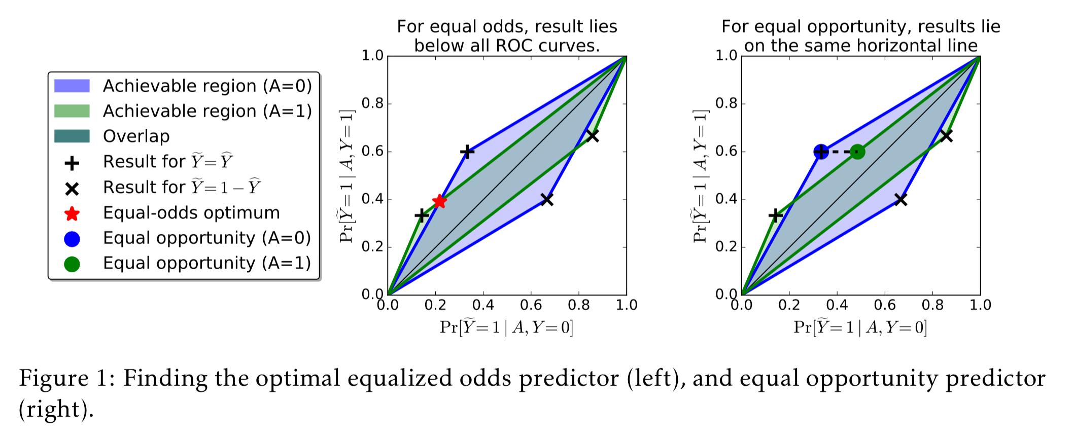
Section 4.2 shows how to extend the method to work with a thresholded score function (as in the FICO example).

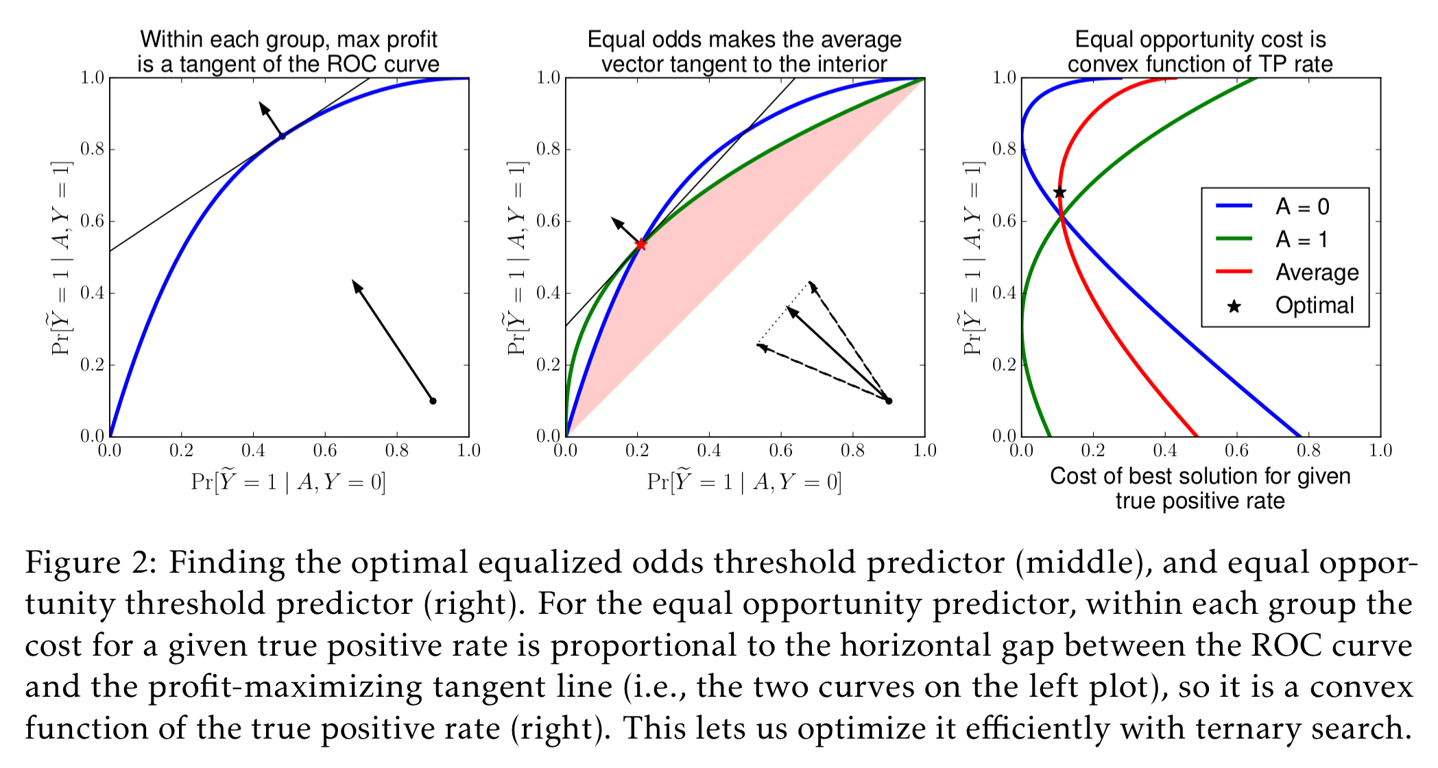
See the full paper for details of the methods.

Limitations

Section 6 in the paper points out that it is possible for two scenarios to be indistinguishable from their joint distribution, and yet have fundamentally different interpretations from the point of view of fairness. No oblivious test can resolve which of the two scenarios applies.

We envision our framework as providing a reasonable way of discovering and measuring potential concerns that require further scrutiny. We believe that resolving fairness concerns is ultimately impossible without substantial domain-specific investigation.

Discussion

Requiring equalized odds aligns incentives such that the entity building the predictor is motivated to achieve fairness. Getting better predictions under these conditions requires collecting features that more directly capture the target Y, unrelated to its correlation with the protected attribute.

In some situations… the equalized odds predictor can be thought of as introducing some sort of affirmative action: the optimally predictive score R* is shifted based on A. This shift compensates for the fact that, due to uncertainty, the score is in a sense more biased than the target label (roughly, R* is more correlated with A than Y is correlated with A). Informally speaking, our approach transfers the burden of uncertainty from the protected class to the decision maker.