The architectural implications of autonomous driving: constraints and acceleration Lin et al., ASPLOS’18
Today’s paper is another example of complementing CPUs with GPUs, FPGAs, and ASICs in order to build a system with the desired performance. In this instance, the challenge is to build an autonomous self-driving car!
Architecting autonomous driving systems is particularly challenging for a number of reasons…
- The system has to make “correct” operational decisions at all times to avoid accidents, and advanced machine learning, computer vision, and robotic processing algorithms are used to deliver the required high precision. These algorithms are compute intensive.
- The system must be able to react to traffic conditions in real-time, which means processing must always finish under strict deadlines (about 100ms in this work).
- The system must operate within a power budget to avoid negatively impacting driving range and fuel efficiency.
So how do you build a self-driving car?
There are several defined levels of automation, with level 2 being ‘partial automation’ in which the automated system controls steering and acceleration/deceleration under limited driving conditions. At level 3 the automated system handles all driving tasks under limited conditions (with a human driver taking over outside of that). By level 5 the system is fully automated.
The following table shows the automation levels targeted by leading industry participants, together with the platforms and sensors used to achieve this:
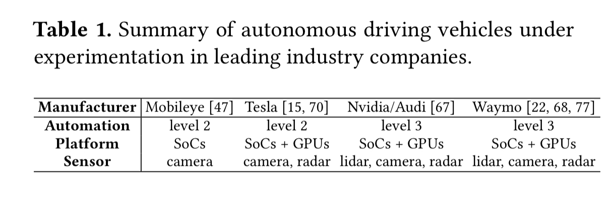
In this work, the authors target highly autonomous vehicles (HAVs), operating at levels 3-5. Moreover, they using vision-based systems using cameras and radar for sensing surroundings, rather than the much more expensive LIDAR.
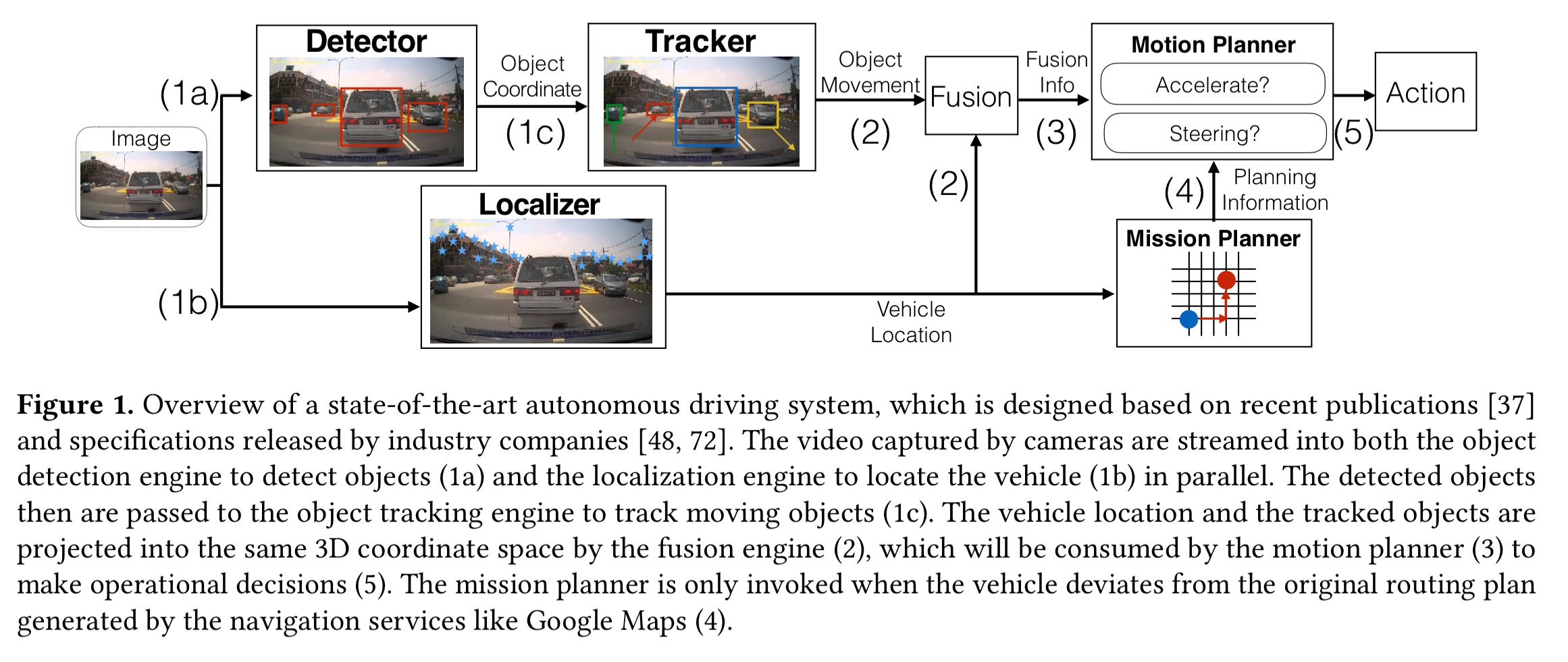
A typical end-to-end autonomous driving system looks something like this:

(Enlarge)
Captured sensor data is fed to an object detector and a localizer (for identifying vehicle location at decimeter-level) in parallel. The object detector identifies objects of interest and passes these to an object tracker to associate the objects with their movement trajectory over time. The object movement information from the object tracker and the vehicle location information from the localizer is combined and projected onto the same 3D coordinate space by a sensor fusion engine.
The fused information is used by the motion planning engine to assign path trajectories (e.g. lane change, or setting vehicle velocity). The mission planning engine calculates the operating motions needed to realise planned paths and determine a routing path from source to destination.
Due to the lack of a publicly available experimental framework, we build an end-to-end workload to investigate the architecture implications of autonomous driving vehicles.
For each of the six main algorithmic components (object detection, object tracking, localization, fusion, motion planning, and mission planning), the authors identify and select state of the art algorithms.
Object detection
For object detection, the YOLO DNN-based detection algorithm is used.
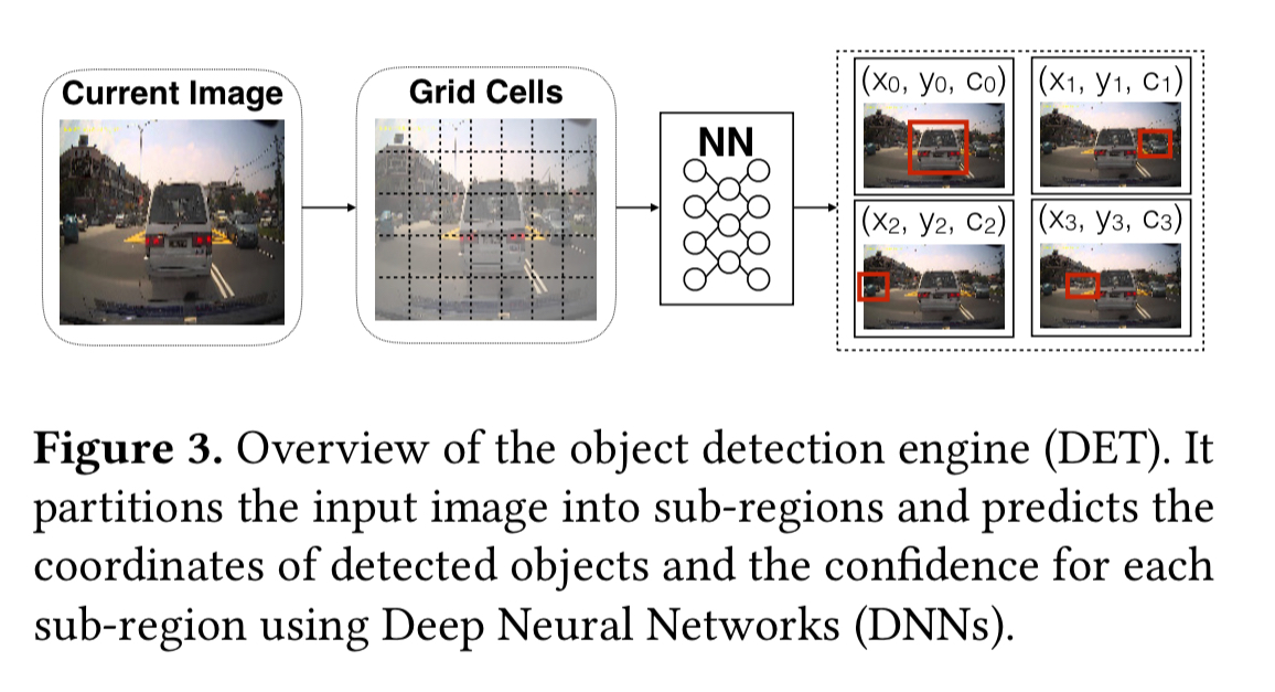
Object detection is focused on the four most important categories for autonomous driving: vehicles, bicycles, traffic signs, and pedestrians.
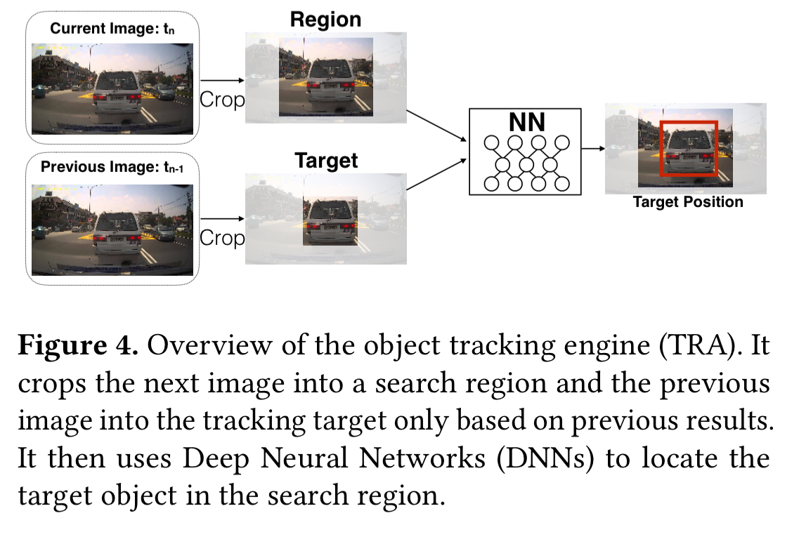
Object tracking
GOTURN (also DNN-based) is used for object tracking. GOTURN tracks a single object, so a pool of trackers are used.
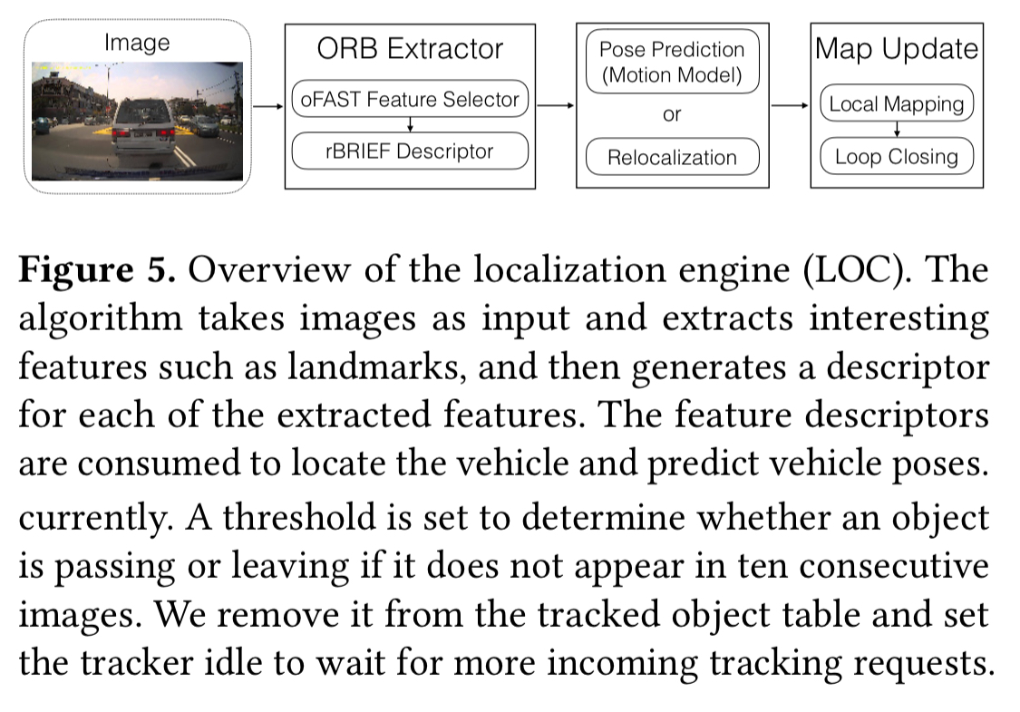
Localization
For localization ORB-SLAM is used, which gives high accuracy and can also localize the vehicle regardles of viewpoint.
Fusion
No reference is given for the fusion engine component, but it is comparatively simple compared to the other components, and perhaps was custom built for the project. It combines the coordinates of tracked objects from the GOTURN trackers with the vehicle position from ORB-SLAM and maps them onto the same 3D-coordinate space to be sent to the motion planning engine.
Motion & Mission planning
Both motion and mission planning components come from the Autoware open-source autonomous driving framework. Motion planning is done using graph-based search to find minimum cost paths when the vehicle is in large open spaces like parking lots or rural areas, in more structured areas ‘conformal lattices with spatial and temporal information’ are used to adapt the motion plan to the environment. Mission planning uses a rule-based approach combining traffic rules and the driving area condition, following routes generated by navigation systems such as Google Maps. Unlike the other components which execute continuously, mission planning is only executed once unless the vehicle deviates from planned routes.
Constraints
How quickly an autonomous system can react to traffic conditions is determined by the frame rate (how fast we can feed real-time sensor data into the process engine), and the processing latency (how long it takes us to make operational decisions based on the captured sensor data). The fastest possible action by a human driver takes 100-150ms (600-850ms is more typical). The target for an autonomous driving system is set at 100ms.
An autonomous driving system should be able to process current traffic conditions within a latency of 100ms at a frequency of at least once every 100ms.
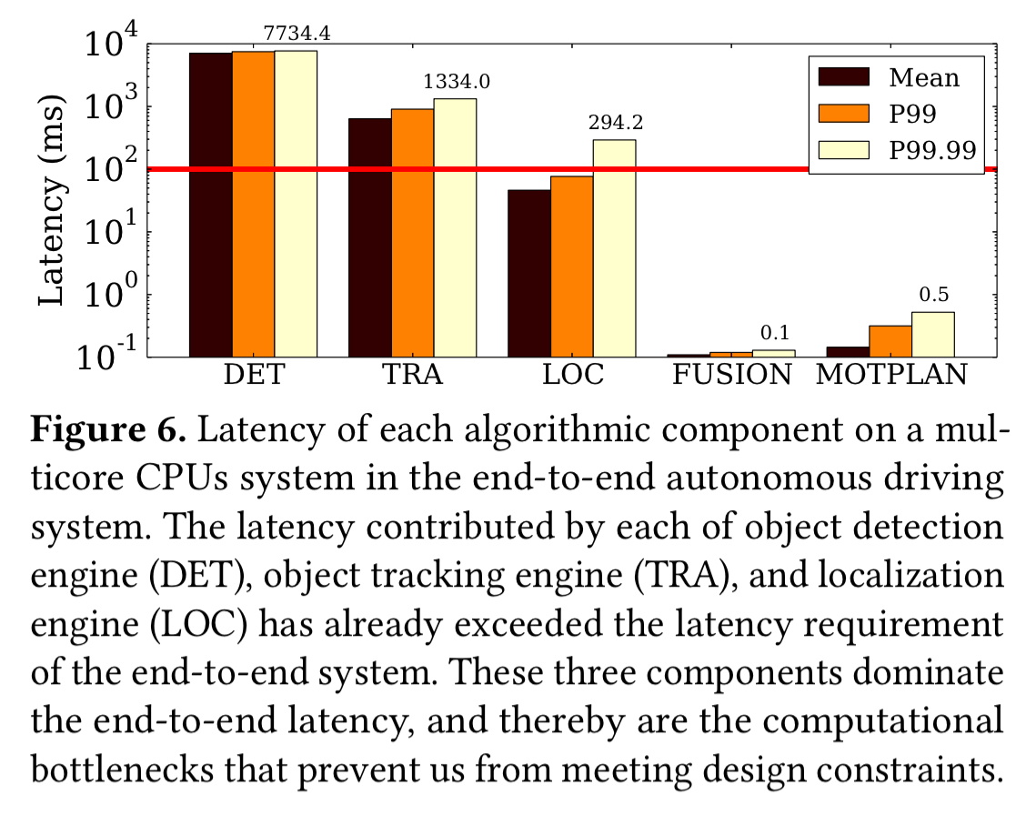
The system also needs extremely predictable performance, which means that long latencies in the tail are unacceptable. Thus 99th, or 99.99th, percentile latency should be used to evaluate performance.
All those processors kick out a lot of heat. We need to keep the temperature within the operating range of the system, and we also need to avoid overheating the cabin. This necessitates additional cooling infrastructure.
Finally, we need to keep an eye on the overall power consumption. A power-hungry system can degrade vehicle fuel efficiency by us much as 11.5%. The processors themselves contribute about half of the additional power consumption, the rest is consumed by the cooling overhead, and the storage power costs of storing tens of terabytes of map information.
With the CPU-only baseline system (16-core Intel Xeon at 3.2GHz), we can clearly see that three of the key components: object detection, tracking, and localisation, do not meet the 100ms individually, let alone when combined.
Beyond CPUs
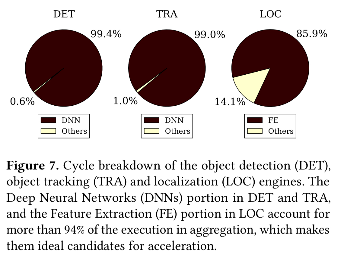
Looking further into these three troublesome components, we can see that DNN execution is the culprit in detecting and tracking, and feature extraction takes most of the time in localisation.
…conventional multicore CPU systems are not suitable to meet all the design constraints, particularly the real-time processing requirement. Therefore, we port the critical algorithmic components to alternative hardware acceleration platforms, and investigate the viability of accelerator-based designs.
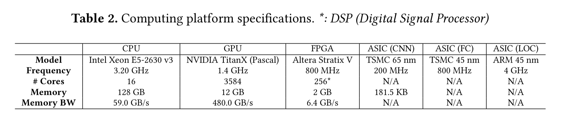
The bottleneck algorithmic components are ported to GPUs using existing machine learning software libraries. YOLO is implemented using the cuDNN library from Nvidia, GOTURN is ported using Caffe (which in turn using cuDNN), and ORB-SLAM is porte to GPUs using the OpenCV library.
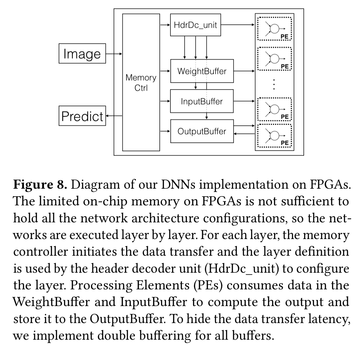
FPGA optimised versions of DNN and feature extraction are built using the Altera Stratix V platform.
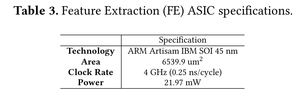
Previously published ASIC implementations are used for DNNs, and a feature extraction ASIC is designed using Verilog and synthesized using the ARM Artisam IBM SOI 45nm library.
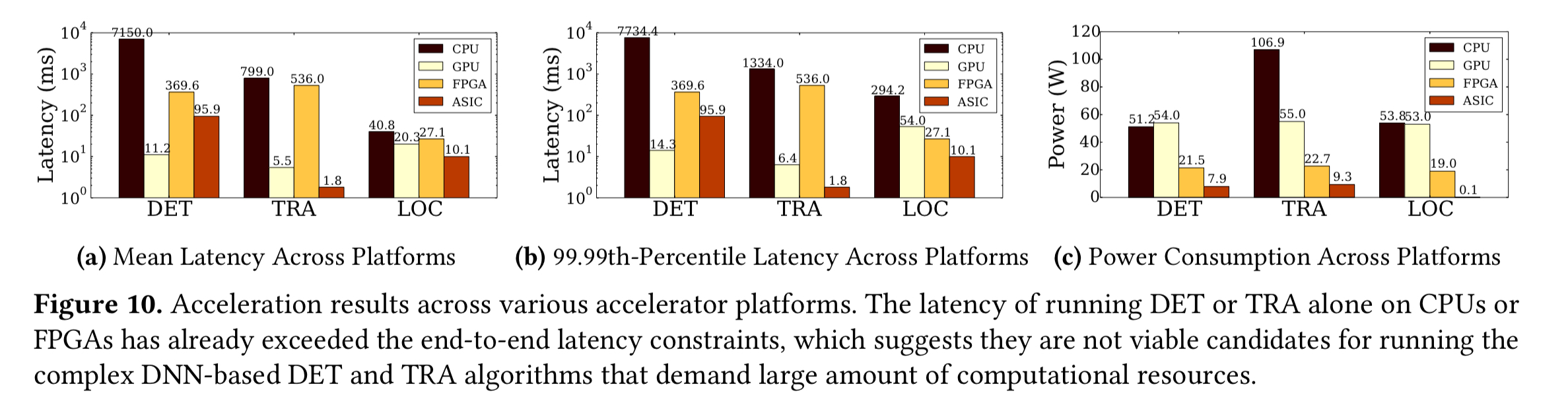
Here’s how the CPU, GPU, FPGA, and ASIC implementations compare for latency and power across the three components:

(Enlarge)
This analysis immediately rules out CPUs and FPGAs for the detection and tracking components, because they don’t meet the tail latency target. Note also that specialized hardware platforms such as FPGAs and ASCIs offer significantly higher energy efficiency.
The perfect blend?
You can use different combinations of CPU, GPU, FPGA, and ASIC for the three different components, in an attempt to balance latency and power consumption. Focusing just on latency for the moment, this chart shows the 99.99th percentile latency for various combinations:
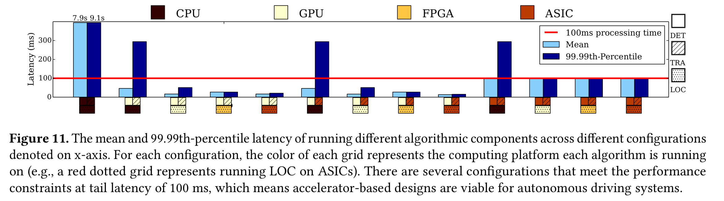
(Enlarge)
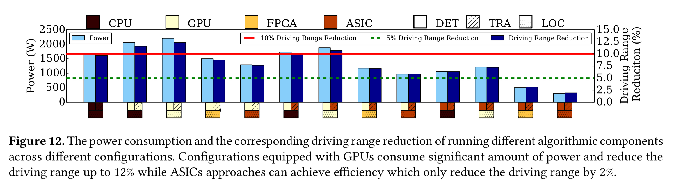
The lowest tail latency of all comes when using GPU-based object detection, and ASICs for tracking and localisation. If we look at power consumption though, and target a maximum of 5% driving range reduction, then we can see that this particular combination is slightly over our power budget.

(Enlarge)
The all-ASIC or ASIC + FPGA-based localisation are the only combinations that fit within the 5% range-reduction budget, and also (just!) meet the latency budget.
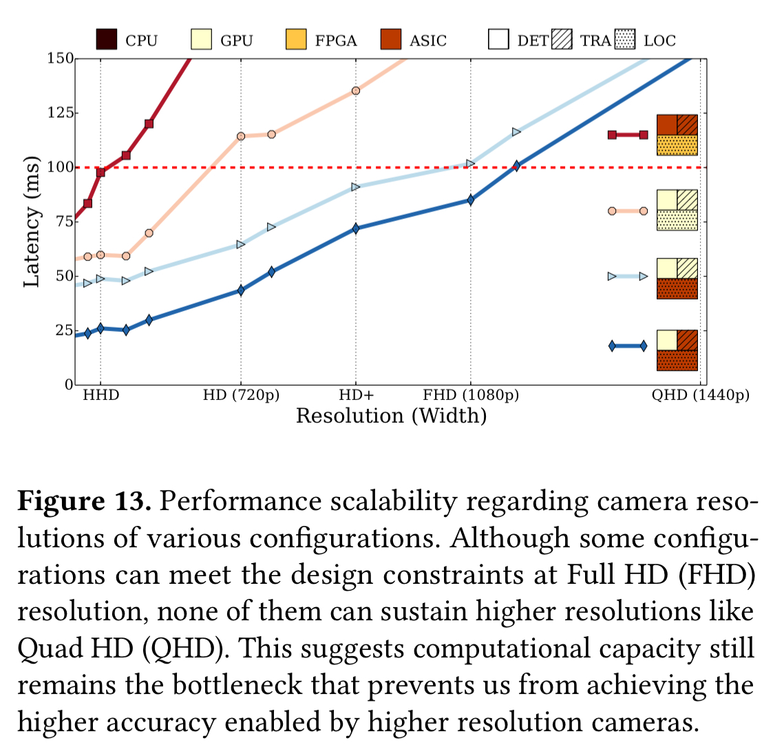
Higher resolution cameras can significantly boost the accuracy of autonomous driving systems. The authors modified their benchmarks to look at end-to-end latency as a function of input camera resolution. Some of the ASCI and GPU accelerated systems can still meet the real-time performance constraints at Full HD resolution (1080p), but none of them can sustain Quad HD: computational capability still remains the bottleneck preventing us from benefiting from higher resolution cameras.
The last word
We show that GPU- FPGA- and ASCI-accelerated systems can reduce the tail latency of [localization, object detection, and object tracking] algorithms by 169x, 10x, and 93x respectively… while power-hungry accelerators like GPUs can predictably deliver the computation at low latency, their high power consumption, further magnified by the cooling load to meet the thermal constraints, can significantly degrade the driving range and fuel efficiency of the vehicle.

Really cool !
I am interested in Ai and have started a coding blog. Here’s the link –
https://myprogrammingadventures123.wordpress.com/
I would love to get some feedback ! Thanks