Opening the black box of deep neural networks via information Schwartz-Viz & Tishby, ICRI-CI 2017

Yesterday we looked at the information theory of deep learning, today in part II we’ll be diving into experiments using that information theory to try and understand what is going on inside of DNNs. The experiments are done on a network with 7 fully connected hidden layers, and widths 12-10-7-5-4-3-2 neurons.

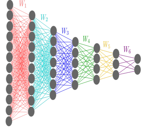
The network is trained using SGD and cross-entropy loss function, but no other explicit regularization. The activation functions are hyperbolic tangent in all layers but the final one, where a sigmoid function is used. The task is to classify 4096 distinct patterns of the input variable into one of two output classes. The problem is constructed such that bits.

Output activations are discretised into 30 bins, and the Markov chain is used to calculate the joint distributions for every hidden layer . Using the joint distributions, it is then possible to calculate the encoder and decoder mutual information, and , for each hidden layer in the network. The calculations were repeated 50 times over, with different random initialisation of network works and different random selections of training samples.

A phase shift during training

We can plot the mutual information retained in each layer on a graph. The following chart shows the situation before any training has been done (i.e., random initial weights of each of the 50 generated networks).

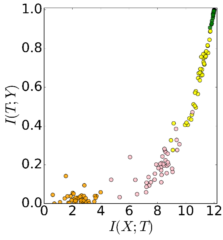
The different colours in the chart represent the different hidden layers (and there are multiple points of each colour because we’re looking at 50 different runs all plotted together). On the x-axis is , so as we move to the right on the x-axis, the amount of mutual information between the hidden layer and the input increases. On the y-axis is , so as we move up on the y-axis, the amount of mutual information between the hidden layer and the output increases.

I’m used to thinking of progressing through the network layers from left to right, so it took a few moments for it to sink in that it’s the lowest layer which appears in the top-right of this plot (maintains the most mutual information), and the top-most layer which appears in the bottom-left (has retained almost no mutual information before any training). So the information path being followed goes from the top-right corner to the bottom-left traveling down the slope.

Part-way through training (here at 400 epochs), we can see that much more information is being retained through the layers .

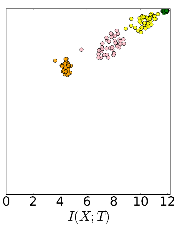
After 9000 epochs we’re starting to see a pretty flat information path, which means that we’re retaining mutual information needed to predict all the way through the network layers.

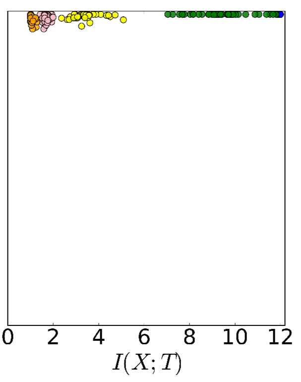
Something else happens during training though, and the best demonstration of it is to be found in watching this short video.

[youtube https://www.youtube.com/watch?v=q45lPv9rev0&w=560&h=315]

What you should hopefully have noticed is that early on the points shoot up and to the right, as the hidden layers learn to retain more mutual information both with the input and also as needed to predict the output. But after a while, a phase shift occurs, and points move more slowly up and to the left.

The following chart shows the average layer trajectories when training with 85% of the data, giving a static representation of the same phenomenon. The green line shows the phase change point, and the yellow points are the final positions.

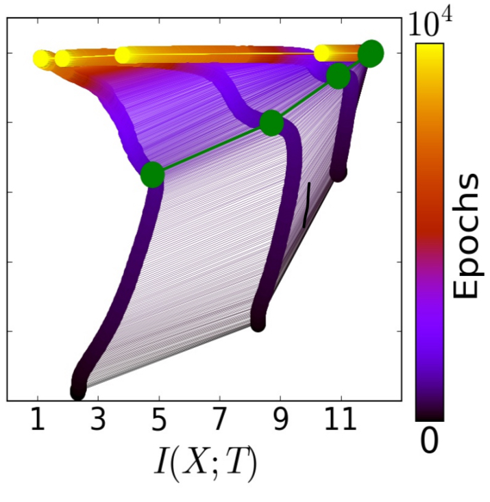
The two optimization phases are clearly visible in all cases. During the fast — Empirical eRror Minimization (ERM) — phase, which takes a few hundred epochs, the layers increase information on the labels (increase ) while preserving the DPI order (lower layers have higher information). In the second and much longer training phase the layer’s information on the input, , decreases and the layers lose irrelevant information until convergence (the yellow points). We call this phase the representation compression phase.

You can also see the phase change clearly (the vertical grey line) when looking at the normalized means and standard deviations of the layer’s stochastic gradients during the optimization process:

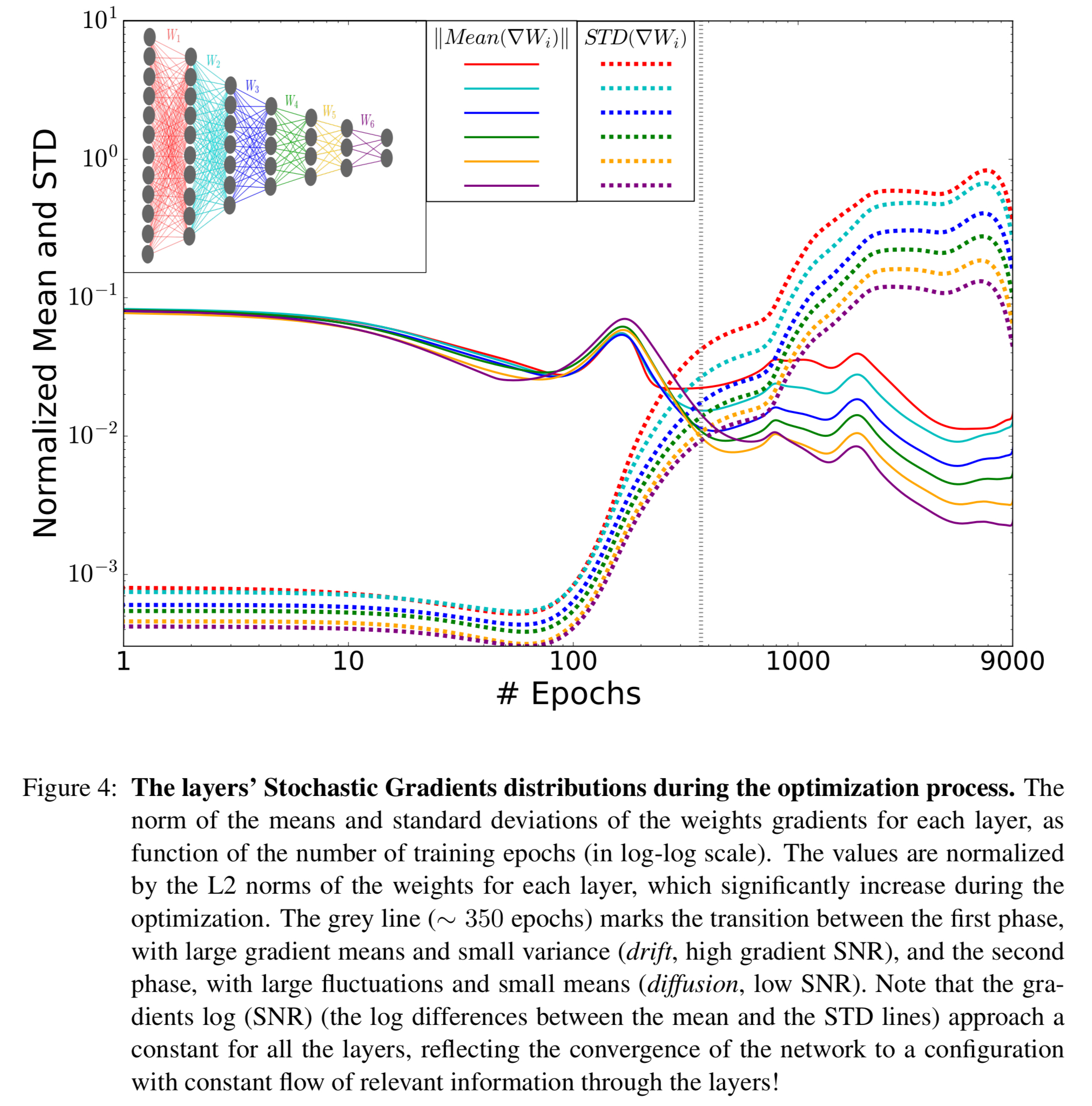
We claim that these distinct SG phases (grey line in the figure above), correspond and explain the ERM and compression phases we observe in the information plane.

The drift phase

The first, ERM, phase is a drift phase. Here the gradient means are much larger than their standard deviations, indicating small gradient stochasticity (high SNR). The increase in is what we expect to see from cross-entropy loss minimisation.

The diffusion phase

The existence of the compression phase is more surprising. In this phase the gradient means are very small compared to the batch-to-batch fluctuations, and the gradients behave like Gaussian noise with very small means for each layer (low SNR). This is a diffusion phase.

…the diffusion phase mostly adds random noise to the weights, and they evolve like Weiner processes [think Brownian motion], under the training error or label information constraint.

This has the effect of maximising entropy of the weights distribution under the training error constraint. This in turn minimises the mutual information – in other words, we’re discarding information in that is irrelevant to the task at hand. The fancy name for this process of entropy maximisation by adding noise is stochastic relaxation.

Compression by diffusion is exponential in the number of time steps it takes (optimisation epochs) to achieve a certain compression level (and hence why you see the points move more slowly during this phase).

One interesting consequence of this phase is the randomised nature of the final weights of the DNN:

This indicates that there is a huge number of different networks with essentially optimal performance, and attempts to interpret single weights or even single neurons in such networks can be meaningless.

Convergence to the Information Bottleneck bound

As can be clearly seen in the charts, different layers converge to different points in the information plane, and this is related to the critical slowing down of the stochastic relaxation process near the phase transitions on the Information Bottleneck curve.

Recall from yesterday that the information curve is a line of optimal representations separating the achievable and unachievable regions in the information plane. Testing the information values in each hidden layer and plotting them against the information curve shows that the layers do indeed approach this bound.

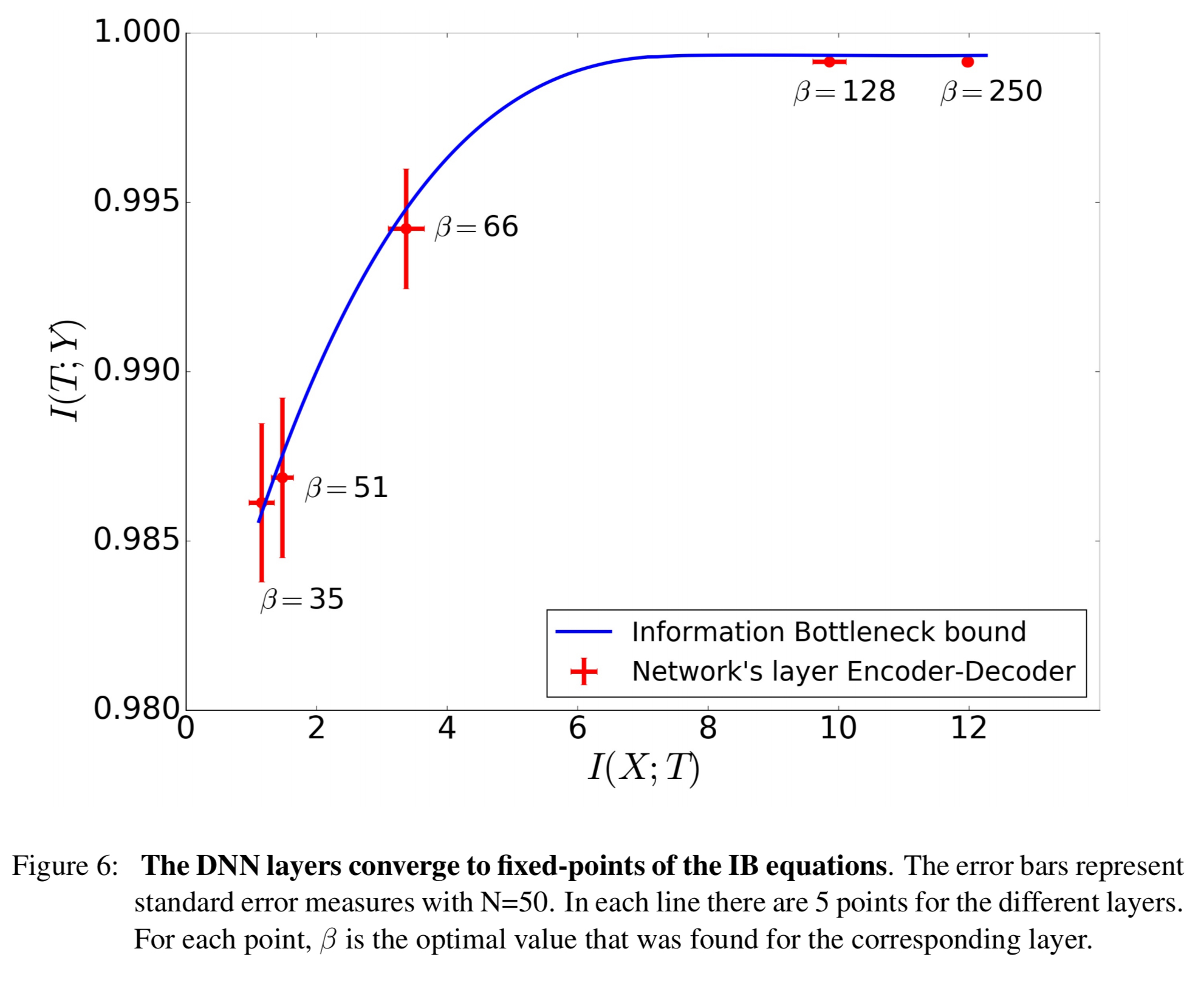
How exactly the DNN neurons capture the optimal IB representations is another interesting issue to be discussed elsewhere, but there are clearly many different layers that correspond to the same IB representation.

Why does deep work so well?

To understand the benefits of more layers the team trained 6 different architectures with 1 to 6 hidden layers and did 50 runs of each as before. The following plots show how the information paths evolved during training for each of the different network depths:

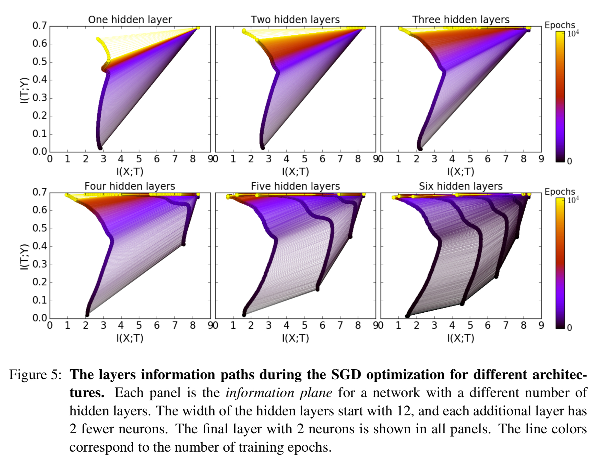
From this we can learn four very interesting things:

1. Adding hidden layers dramatically reduces the number of training epochs for good generalization. One hidden layer was unable to achieve good values even after 10^4 iterations, but six layers can achieve full relevant information capture after just 400.
2. The compression phase of each layer is shorter when it starts from a previous compressed layer. For example, the convergence is much slower with 4 layers than with 5 or 6.
3. The compression is faster for the deeper (narrower and closer to the output) layers. In the diffusion phase the top layers compress first and “pull” the lower layers after them. Adding more layers seems to add intermediate representations which accelerate compression.
4. Even wide layers eventually compress in the diffusion phase. Adding extra width does not help.

Training sample size

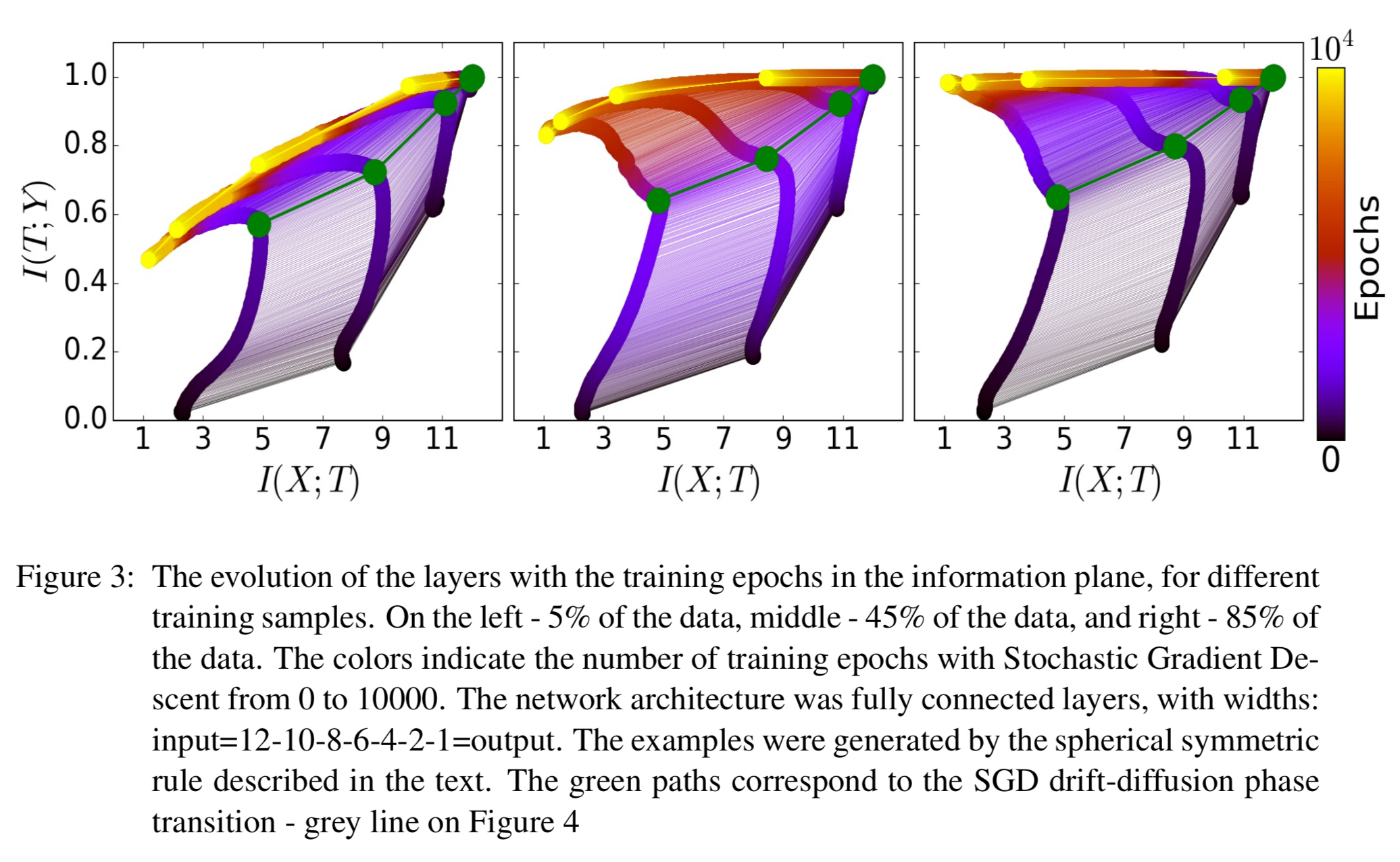
Training sample size seems to have the biggest impact on what happens during the diffusion phase. Here are three charts showing the information paths when training with 5% (left), 45% (middle), and 85% (right of the data):

What does all this tell us about future directions for DL?

We are currently working on new learning algorithms that utilize the claimed IB optimality of the layers. We argue that SGD seems an overkill during the diffusion phase, which consumes most of the training epochs, and the much simpler optimization algorithms, such as Monte-Carlo relaxations, can be more efficient.

Furthermore, the analytic connections between encoder and decoder distributions can be exploited during training: combining the IB iterations with stochastic relaxation methods may significantly boost DNN training.

To conclude, it seems fair to say, based on our experiments and analysis, that Deep Learning with DNN are in essence learning algorithms that effectively find efficient representations that are approximate minimal statistics in the IB sense. If our findings hold for general networks and tasks, the compression of the SGD and the convergence of the layers to the IB bound can explain the phenomenal success of Deep Learning.