Opening the black box of deep neural networks via information Schwartz-Viz & Tishby, ICRI-CI 2017
In my view, this paper fully justifies all of the excitement surrounding it. We get three things here: (i) a theory we can use to reason about what happens during deep learning, (ii) a study of DNN learning during training based on that theory, which sheds a lot of light on what is happening inside, and (iii) some hints for how the results can be applied to improve the efficiency of deep learning – which might even end up displacing SGD in the later phases of training.
Despite their great success, there is still no comprehensive understanding of the optimization process or the internal organization of DNNs, and they are often criticized for being used as mysterious “black boxes”.
I was worried that the paper would be full of impenetrable math, but with full credit to the authors it’s actually highly readable. It’s worth taking the time to digest what the paper is telling us, so I’m going to split my coverage into two parts, looking at the theory today, and the DNN learning analysis & visualisations tomorrow.
An information theory of deep learning
Consider the supervised learning problem whereby we are given inputs and we want to predict labels
. Inside the network we are learning some representation
of the input patterns, that we hope enables good predictions. We also want good generalisation, not overfitting.
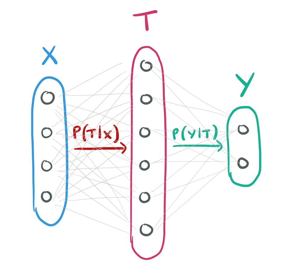
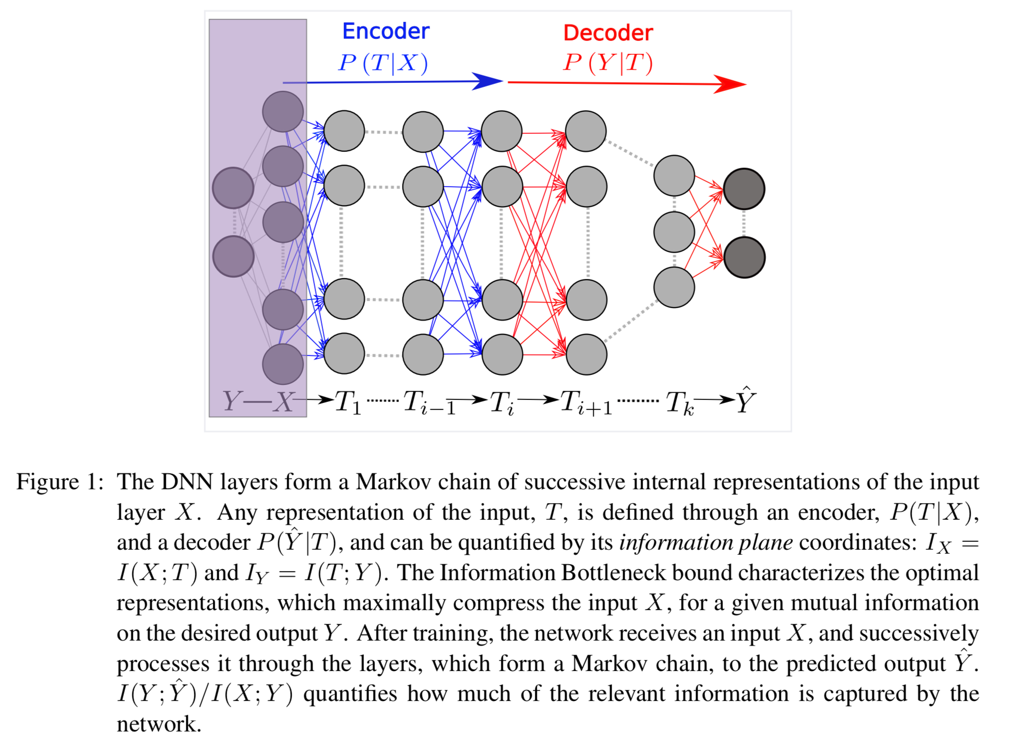
Think of a whole layer as a single random variable. We can describe this layer by two distributions: the encoder
and the decoder
.

So long as these transformations preserve information, we don’t really care which individual neurons within the layers encode which features of the input. We can capture this idea by thinking about the mutual information of with the input
and the desired output
.
Given two random variables and
, their mutual information
is defined based on information theory as
Where is the entropy of
and
is the conditional entropy of
given
.
The mutual information quantifies the number of relevant bits that the input
contains about the label
, on average.
If we put a hidden layer between
and
then
is mapped to a point in the information plane with coordinates
. The Data Processing Inequality (DPI) result tells us that for any 3 variables forming a Markov chain
we have
.
So far we’ve just been considering a single hidden layer. To make a deep neural network we need lots of layers! We can think of a Markov chain of K-layers, where denotes the
hidden layer.

In such a network there is a unique information path which satisfies the DPI chains:
and
Now we bring in another property of mutual information; it is invariant in the face of invertible transformations:
for any invertible functions and
.
And this reveals that the same information paths can be realised in many different ways:
Since layers related by invertible re-parameterization appear in the same point, each information path in the plane corresponds to many different DNN’s , with possibly very different architectures.
Information bottlenecks and optimal representations
An optimal encoder of the mutual information would create a representation of a minimal sufficient statistic of
with respect to
. If we have a minimal sufficient statistic then we can decode the relevant information with the smallest number of binary questions. (That is, it creates the most compact encoding that still enables us to predict
as accurately as possible).
The Information Bottleneck (IB) tradeoff Tishby et al. (1999) provides a computational framework for finding approximate minimal sufficient statistics. That is, the optimal tradeoff between the compression of and the prediction of
.
The Information Bottleneck tradeoff is formulated by the following optimization problem, carried independently for the distributions,
, with the Markov chain:

where the Lagrange multiplier determines the level of relevant information captured by the representation
.
The solution to this problem defines an information curve: a monotonic concave line of optimal representations that separates the achievable and unachievable regions in the information plane.
Noise makes it all work
Section 2.4 contains a discussion on the crucial role of noise in making the analysis useful (which sounds kind of odd on first reading!). I don’t fully understand this part, but here’s the gist:
The learning complexity is related to the number of relevant bits required from the input patterns
for a good enough prediction of the output label
, or the minimal
under a constraint on
given by the IB.
Without some noise (introduced for example by the use of sigmoid activation functions) the mutual information is simply the entropy independent of the actual function we’re trying to learn, and nothing in the structure of the points
gives us any hint as to the learning complexity of the rule. With some noise, the function turns into a stochastic rule, and we can escape this problem. Anyone with a lay-person’s explanation of why this works, please do post in the comments!
Setting the stage for Part II
With all this theory under our belts, we can go on to study the information paths of DNNs in the information plane. This is possible when we know the underlying distribution and the encoder and decoder distributions
and
can be calculated directly.
Our two order parameters,
and
, allow us to visualize and compare different network architectures in terms of their efficiency in preserving the relevant information in
.
We’ll be looking at the following issues:
- What is SGD actually doing in the information plane?
- What effect does training sample size have on layers?
- What is the benefit of hidden layers?
- What is the final location of hidden layers?
- Do hidden layers form optimal IB representations?
Have you found how to calculate this I(X,T_i) in practice, say, for MNIST and FC layers?
In section 2.5 of the paper, the authors describe the criteria under which this can be done. They only do so for a strictly controlled environment, leaving the more general case to future work – though they give some hints: “As proposed by Tishby and Zaslavsky (2015), we study the information paths of DNNs in the information plane. This can be done when the underlying distribution, P (X, Y ), is known and the encoder and decoder distributions P (T |X ) and P (Y |T ) can be calculated directly. For ”large real world” problems these distributions and mutual information values should be estimated from samples or by using other modeling assumptions. Doing this is beyond the scope of this work, but we are convinced that our analysis and observations are general, and expect the dynamics phase transitions to become even sharper for larger networks, as they are inherently based on statistical ensemble properties. Good overviews on methods for mutual information estimation can be found in Paninski (2003) and Kraskov et al. (2004).”
Found this solution https://arxiv.org/abs/1705.02436
from this link: https://openreview.net/forum?id=ry_WPG-A-
Thank you so much for reviewing this topic! You mention “If we put a hidden layer T between X and Y then T is mapped to a point in the information plane with coordinates (I(X;T), I(T;Y))”
I’m not yet very familiar with Information Theory beyond entropy. What does the information plane mean? And what does it mean to map a point in the information plane with some coordinates? This topic is really fascinating!
By information plane here, the authors are referring (as I understand it!), to the 2D plane created with the mutual information between the input and the hidden layer on the x-axis, and the mutual information between the output and the hidden layer on the y-axis. Another way of thinking about what this phrase means is just “when we think about what’s happening inside of the neural network in terms of information…”. Part II (posted tomorrow) contains a number of example plots etc., that will hopefully help to make all this a little clearer.
Looking forward to it! Thanks a lot for this review, reading someone else’s perspective helps. I still need to wrap my head around the whole idea of information theory
Great post. Do you know of any other blogs/podcasts/youtube channels doing something similar to your morning paper, or 2 minute papers on youtube but in other fields ?
It’s a great idea, I’d love to be introduced the gist of papers from fields outside of computer science.
About adding noise to a model, if it’s the same concept that I envision, you’d be adding extra bits to an existential set of data to generalize the data structure for pattern recognition. It might help to take an example, It’s like adding noise to a clear photo in Photoshop, if you use the filter to add noise to a picture you see more blocked edges on the photo, this allows for more generalized manipulations of the image because extra bits are added onto the smooth edges. A graphics artist can add effects to an image because the separations become more distinct between objects.
I meant existing instead existential.
Quote: “… Without some noise (introduced for example by the use of sigmoid activation functions) …”
I do not see how sigmoid functions could introduce noise by them selves. The way I see it is more: the noise is introduced by the random initialization of the parameters, the variance of this noise is THEN amplified by the sigmoid function (or any other non-linearity).
That part of the paper (not present in the Researchgate version) is pretty foggy to me too. However, the way I **understand** it is that, yes, the noise is generated “by the sigmoids themselves” if you consider “noise” the various values of the sigmoid (wobbling between 0 and 1 as you evaluate the various input); that wobbling could be interpreted as a distance of an input x to the decision boundary and, at the same time, considered as noise as opposite to, for instance, a binary function that just labels as ‘0’ or ‘1’ depending on which side of the decision boundary an input lies.
The reason (I think) for all this is to say that as the neural networks in the paper example are equipped with sigmoids, a theory based on information can tell us something about the classification complexity.
Not sure what is going to happen when a different nonlinearity is used at the neurons instead of a sigmoid. For instance, if a ReLu is used (as very common in deep networks) the distance concept doesn’t quite work: then I am unclear if insights on the classification complexity can be provided by an information-based approach.
Can you please elaborate how invertible functions help us determine that same information path can be realized in many different ways?
Here’s my interpretation: suppose we have a function g :: X -> X’, and a function h :: Y -> Y’. Then the mutual information between X and Y is the same as the mutual information between g(X) and h(Y), iff those functions are invertible. That is, I can define g’ :: X’ -> X such that g’(g(x)) == x. Intuitively to me this must be the case, since if the function is invertible (I can always go back to the original) it must be that I haven’t lost any information. And likewise the function g() can’t conjure up new information out of thin air!
Now, the functions g() and h() that I chose above are arbitrary. We could make lots of different choices of g() and h() so long as they retained the invertibility property. Now think of those functions as transformations at a layer in the network, and we have lots of different potential networks that share the same properties in the information plane.
Hi,
can anyone tell me why minimizing I(X,X’) corresponds to (lossy) compression? Couldn’t this just be that information is arbitrarily ‘destroyed’?