Peeking at A/B tests: why it matters, and what to do about it Johari et al., KDD’17
and
Continuous monitoring of A/B tests without pain: optional stopping in Bayesian testing Deng, Lu, et al., CEUR’17
Today we have a double header: two papers addressing the challenge of monitoring ongoing experiments. Early stopping in traditional A/B testing can really mess up your results. Yet it’s human nature to want to look at how things are going, and if we can get answers more quickly, surely that would be better?
‘Peeking at A/B tests: why it matters and what to do about it’ provides a great explanation of the issues, and presents a solution in the classic Null Hypothesis Statistical Testing (NHST) framework. Their solution, called mSPRT, the mixture sequential probability ratio test, has been part of the Optimizely platform since January 2015.
‘Continuous monitoring of A/B tests without pain: optional stopping in Bayesian testing’ provides us with an alternative. NHST is a frequentist viewpoint, does Bayes offer a different way of thinking about the problem? There’s a certain intuitiveness about this to me, though I’ve learned the hard way that intuition can be dangerous in probability and statistics! We have a prior estimate of the likelihood that our experiment will have a beneficial impact. When we get a new data point from a sample, our confidence (posterior probability) should go up or down a little bit…
The dangers of peeking at ongoing A/B tests
The validity of p-values and confidence intervals in traditional A/B testing requires that the sample sized be fixed in advance. There is a great temptation though for users to peek at the ongoing results while the experiment is in progress.
Peeking early at results to trade off maximum detection with minimum samples dynamically seems like a substantial benefit of the real-time data that modern A/B testing environments can provide. Unfortunately, stopping experiments in an adaptive manner through continuous monitoring of the dashboard will severely favorably bias the selection of experiments deemed significant.
With for example 10,000 samples, the false positive probability can be inflated by 5-10x! The following chart illustrates the issue. Here we’re looking at a treatment and control that both consist of Normal(0,1) data, and we’re testing the null hypothesis that the mean is the same in both variations.
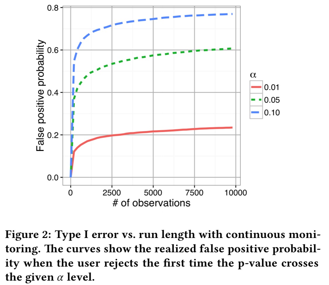
The curves show the realized Type-I error if the null hypothesis is rejected the first time the p-value falls below the given level of 
That means that, throughout the industry, users have been drawing inferences that are not supported by their data.
Optimizely’s solution – mSPRT
The first significant contribution of our paper is the definition of always valid p-values that control Type I error, no matter when the user chooses to stop the test.
The solution builds on the field of sequential analysis in statistics, where sequential tests allow the terminal sample size to be data-dependent. Section 3.2 of the paper establishes a link between sequential tests and always valid p-values that I’m not going to attempt to explain! Sequential analysis traces its roots back to 1945. Given a user’s choice of Type I error constraint (threshold) and a desired balance between power and sample size, it would be possible to simply choose a sequential test from the literature that optimises the objective.
But for an A/B testing platform, there is a fundamental problem with this approach: each user wants a different trade-off between power and sample size!
Optimizely uses a particular family of sequential tests, the mixture sequential probability ratio test (mSPRT) to provide users with the ability to make this trade-off. Details are in section 4 of the paper (and I don’t think I could add any value here by attempting them to explain them to you!).
Early stopping with Bayesian testing
In the Bayesian approach we assume there is a prior probability for the null hypothesis 

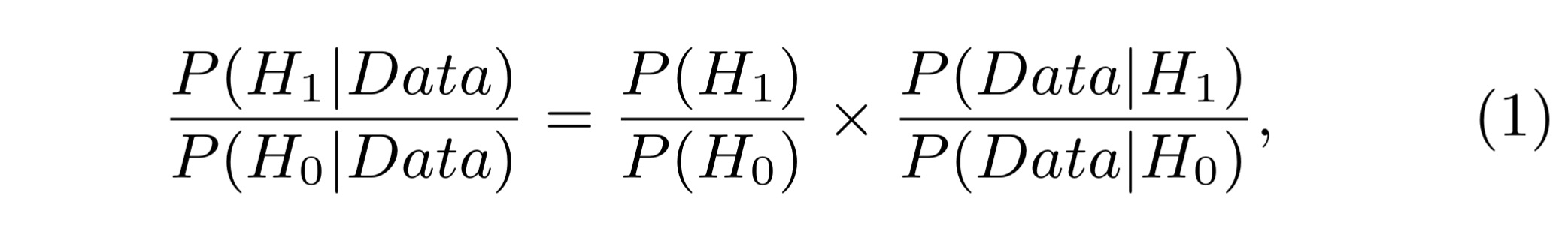
Which can also be expressed simply as: posterior odds = prior odds x Bayes factor. If you’re more used to seeing Bayes’ Rule expressed using probabilities than odds (as I am), then this piece from Maths Better Explained on ‘Understanding Bayes theorem with ratios‘ might help here. Bayesian testing allows us to control the false discovery rate (FDR), the percentage of times we think something is a true discovery, when in fact it isn’t. We need to start out with some prior odds – historical A/B tests can give us these (e.g., the odds that any particular experiment is likely to be successful are about 1 in 3 as reported by Microsoft).
The trouble is, the community were divided over whether or not continuous monitoring is a proper practice in Bayesian testing. If it isn’t, then Bayesian testing still won’t solve the peeking problem.
In this paper, we formally prove the validity of Bayesian testing with continuous monitoring when proper stopping rules are used, and illustrate the theoretical results with concrete simulation illustrations.
The key theorem in the paper shows that early stopping does not change the false discovery rate. There are two conditions: you must use all of the data available to you at the stopping time (no selecting just the bits you like from the history), and you can’t peek into the future.
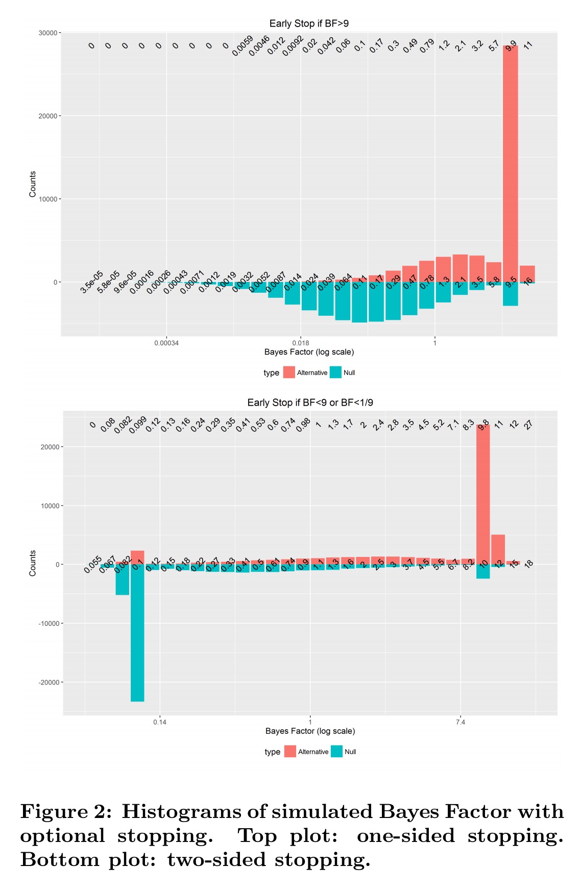
Section 3 of the paper provides the results of a simulation to help you understand why the theorem holds. Section 4 provides the accompanying proof. Below are the results of a simulation with 100,000 runs, and 100 observations in each run. The underlying data has normal distribution N(0.2, 1). The null hypothesis
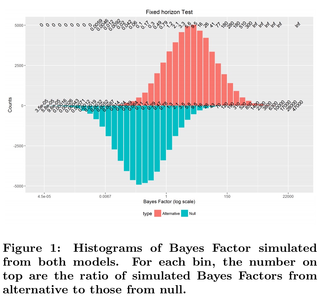
Look for example at the bin for Bayes Factors close to 2.1…
There are about 4000 runs from H1 (height of the red bar) that produced a Bayes Factor close to 2.1 (among 50,000 simulation runs), while around 2000 (height of the blue bar) are from H0. The actual ratio is shown on top of the plot and is 2.1, which is the same as the Bayes Factor we started with.
When we allow early stopping, we see a spike at the stopping Bayes Factor boundary, but the numbers on the top margin – ratios of observed Bayes Factors in each bin from H1 to H0 remain very clone to the theoretical Bayes Factor value calculated… as in a fixed horizon test. This is exactly what Theorem 1 claims, and this simulation study confirms it!
Your three options, and how to choose between them
When it comes to running A/B tests, we now have three basic options:
- If you’re using a traditional A/B testing framework, then as we looked at earlier this week you should decide on the required sample size up front, and avoid any interpretation of results until the test is complete. You may (should!) monitor the ongoing test to look for abnormal metric movements – the purpose of this is to quickly abandon a harmful or buggy test, not to infer anything about the efficacy of the treatment.
- You can use a method which supports early stopping with validity in the context of NHST. Optimizely supports one such method – I haven’t checked all the other options to see if they’ve integrated such a solution yet (maybe we’ll find out in the comments!).
- You can use Bayesian testing.
Putting aside practical considerations, such as whether or not there’s an out-of-the-box offering you can just use, how can we choose between options (2) and (3)? It turns out that there’s no straightforward comparison we can make:
… mSPRT controls Type-I error – the chance of false rejection when [the null hypothesis] is true, while Bayesian test controls False Discovery Rate (FDR) – the chance of false rejection when deciding to reject [the null hypothesis]. There is no simple relationship between the two. When we reject more aggressively, Type-I error will increase, but FDR does not necessarily increase, as long as more aggressive rejection will also reject more true positives.
I had to read that paragraph many times, and consult a few additional resources as well to try and get this straight in my head! Here’s an example:
- with mSPRT (p-values), we can say e.g., ‘there is only a 5% chance that this particular “discovery” is in fact not real.’
- with FDR (q-values), we can say e.g., ‘only 5% of the “discoveries” we make are in fact not real.’
It’s the subtle difference between our confidence in each individual case, and our overall success rate. In a clinical trial for example, we probably want high confidence that we’re not seeing a false positive, and thus controlling Type-I error seems a better bet. If you’re conducting lots and lots of A/B tests though, then perhaps the balance shifts towards Bayesian testing?
If our goal is not to focus on each individual test, but the overall performance of our decision on a large set of tests, and the cost of false rejection and false negative are in the same order, then we believe FDR is a better criterion. Large scale A/B testing platforms are an example of the latter. In an agile environment, where success is built upon a lot of small gains, as long as we are shipping more good features that really meet customer needs than useless ones, we are moving in the right direction.
If you want to go deeper, “Bayesian testing is not immune to optional stopping issues” has a great list of references and discussion points.
Let the debates continue…

4 thoughts on “Peeking at A/B tests: continuous monitoring without pain”
Comments are closed.