Struc2vec: learning node representations from structural identity

struc2vec: learning node representations from structural identity Ribeiro et al., KDD’17

This is a paper about identifying nodes in graphs that play a similar role based solely on the structure of the graph, for example computing the structural identity of individuals in social networks. That’s nice and all that, but what I personally find most interesting about the paper is the meta-process by which the authors go about learning the latent distributed vectors that capture the thing they’re interested in (structural similarity in this case). Once you’ve got those vectors, you can do vector arithmetic, distance calculations, use them in classifiers and other higher-level learning tasks and so on. As word2vec places semantically similar words close together in space, so we want structurally similar nodes to be close together in space.

Recall that for word embeddings we need the context of a word (the other words that appear close to it in sentences) in order to learn a word vector. If we could come up with some similar notion of context for a node in graph, then we could use the same approach. Since we’re interested in similarity based on graph structure, regardless of node and edge labels etc., we’ll make sure that the information we want to ignore doesn’t inform the context in any way. The technique is to create a meta-graph encoding structural information about the graph of interest, and then use random walks starting from each node in the meta-graph to determine the context set.

Problem and high level approach

Structural identity is a concept of symmetry in networks in which nodes are identified based on the network structure. The concept is strongly related to functions or roles played by nodes in the network, an important problem in social and hard sciences.

We want to learn representations that capture the structural identity of nodes in the network, such that:

the distance between the latent representation of nodes is strongly correlated to their structural similarity.
the latent representation does not depend on any non-structural node or edge attribute (e.g., node labels).

Struc2vec has four main steps:

Determine the structural similarity between each vertex pair in the graph, for different neighbourhood sizes.
Construct a weighted multi-layer graph, in which each layer corresponds to a level in a hierarchy measuring structural similarity (think: ‘at this level of zoom, these things look kind of similar’).
Use the multi-layer graph to generate context for each node based on biased random walking.
Apply standard techniques to learn a latent representation from the context given by the sequence of nodes in the random walks.

Let’s now take a closer look at each of those four steps.

A measure of structural similarity

Here’s a graph $G$ with diameter $k^*$ .

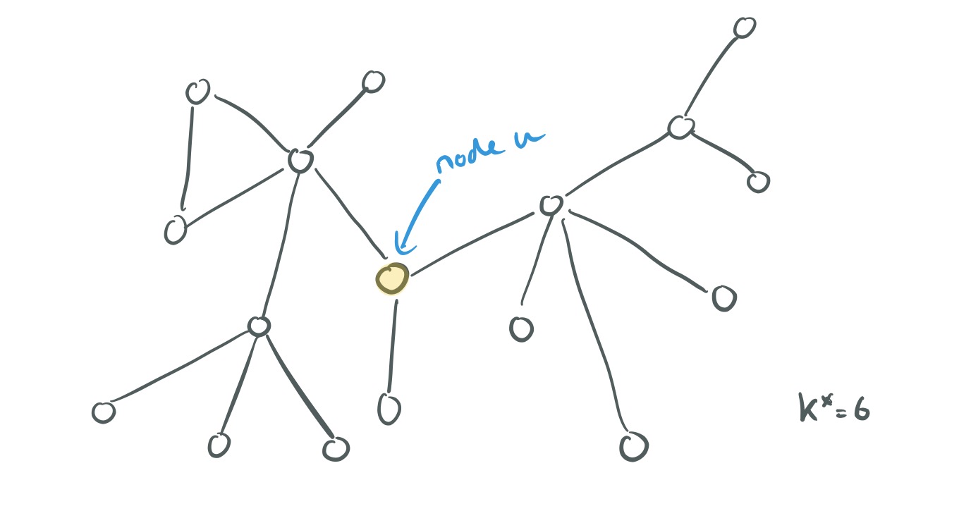
For a node $u$ in the graph, let $R_{k}(u)$ be the set of nodes at radius k (k hops) from $u$ .

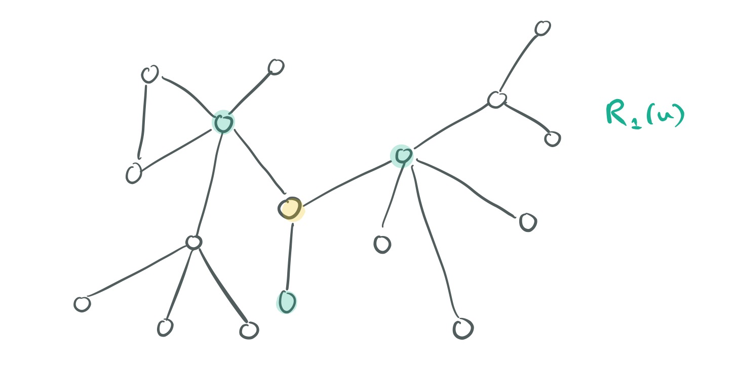
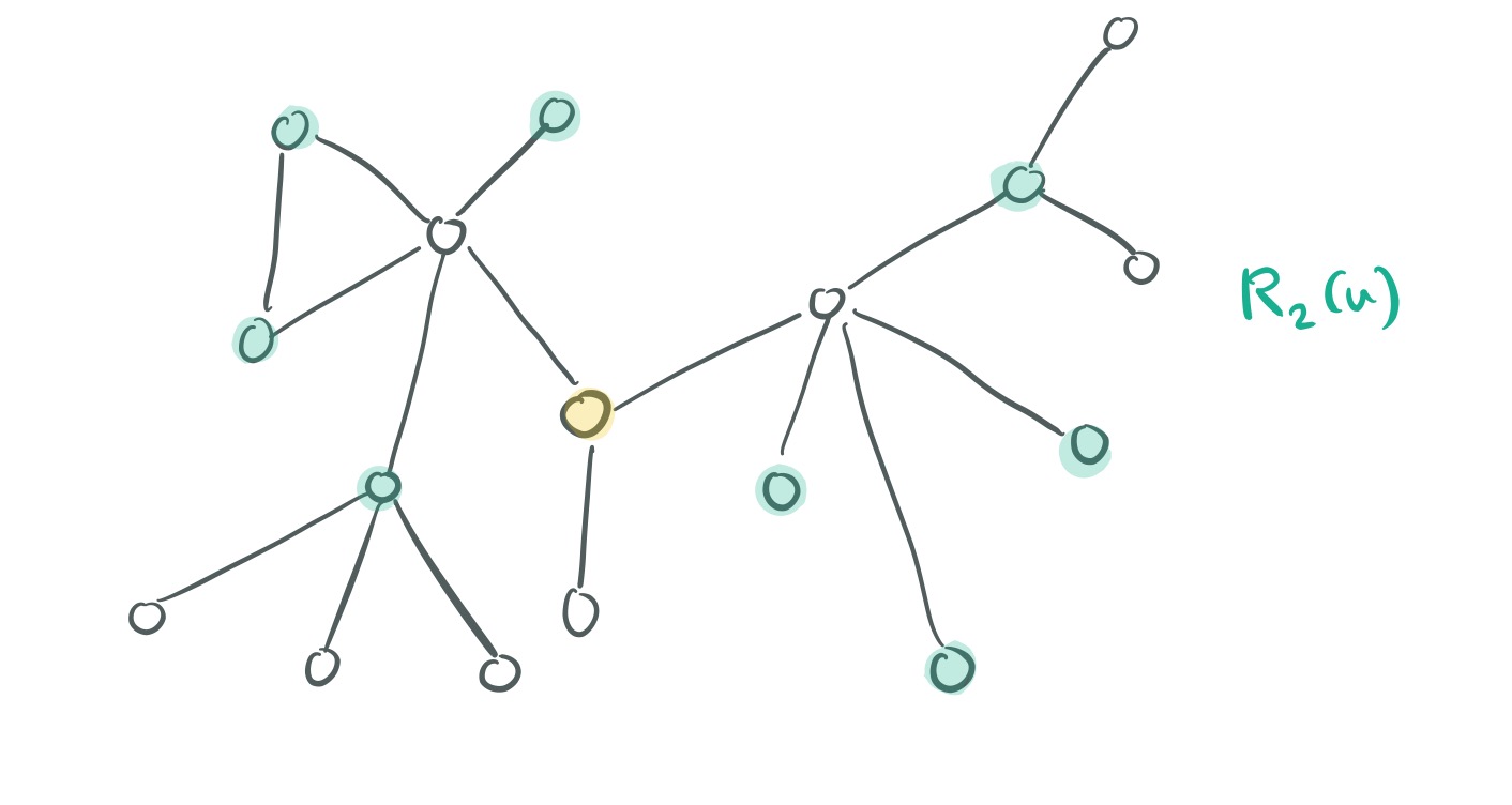
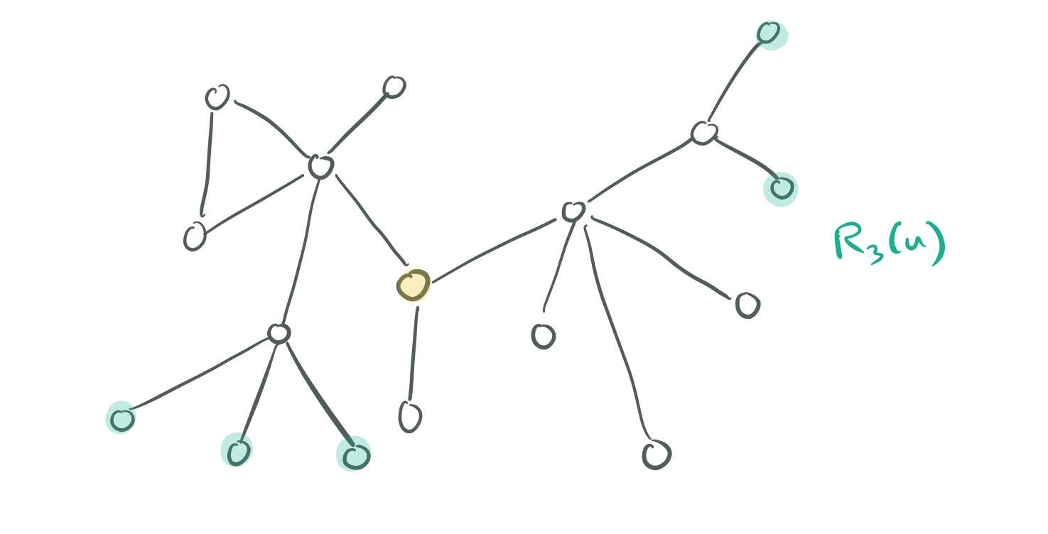
Now, for two nodes $u$ and $v$ , we want to know how similar their structures are for a given value of $k$ . In other words, we want to compute a measure of structural distance for the k-neighbourhoods. Call this distance function $f_{k}(u,v)$ . The function is only defined when both nodes have at least one k-neighbour.

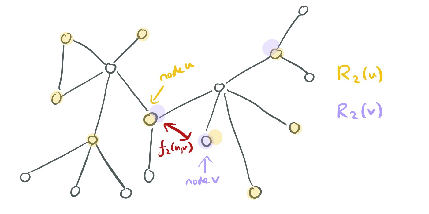
The structural distance $f_{k}(u,v)$ has two components: the distance at the $(k-1)$ -neighbourhood, and the degree sequence distance $g(s(R_k(u)),s(R_k(v)))$ between the ordered degree sequence $s$ of the nodes in k-neighbourhoods of $u$ and $v$ .

$f_{k}(u,v) = f_{k-1}(u,v) + g(s(R_k(u)),s(R_k(v)))$

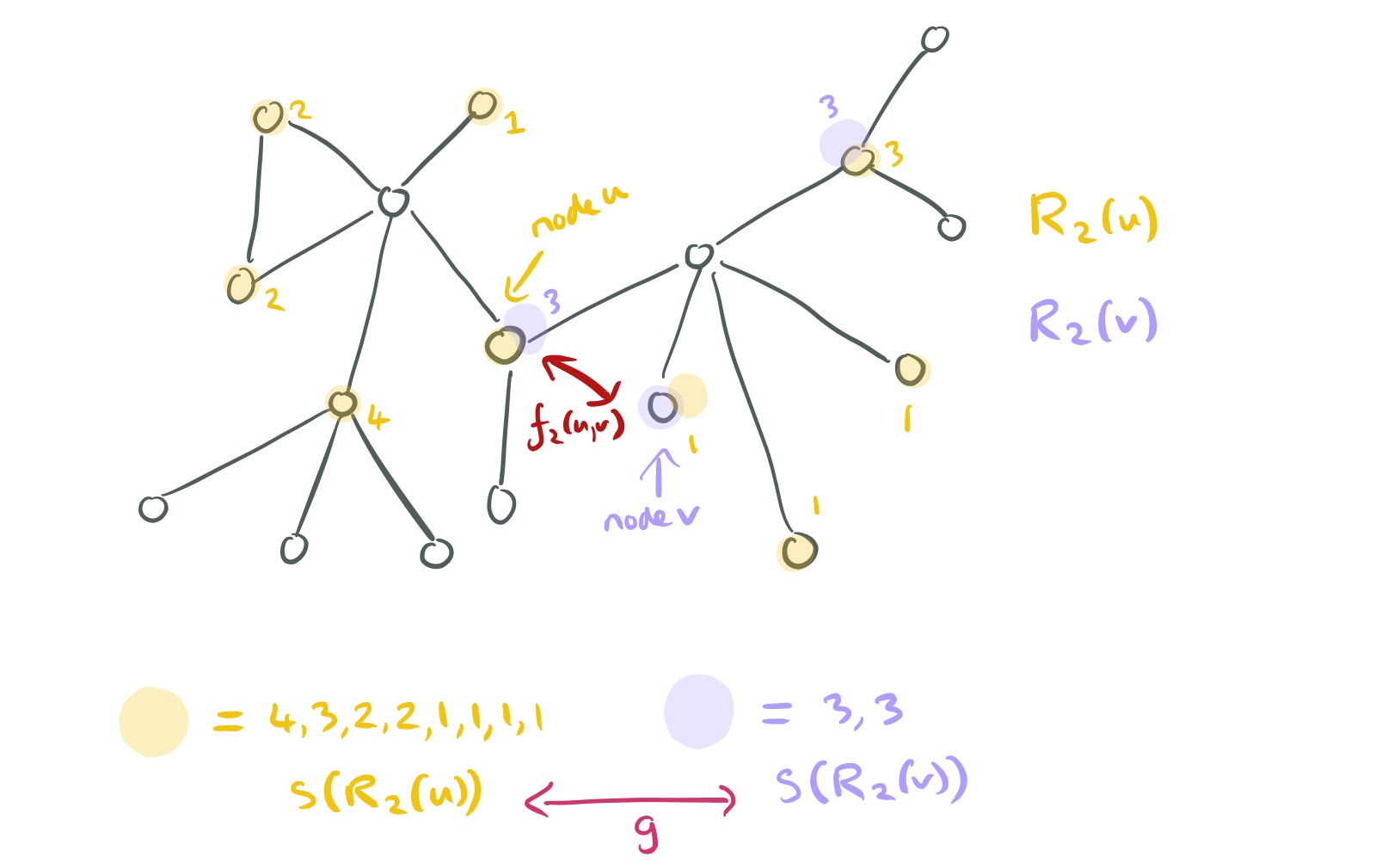
The two degree sequences may be of different sizes, and each element in the sequence will have some value in the range $[0, n-1]$ for an n-node graph. The authors treat these sequences like a timeseries and use DTW (dynamic time warping) to assess their similarity. DTW in turn needs yet another distance function, which computes a distance between matched elements in the first and second sequences. For this, we can use:

$d(a,b) = \frac{\max(a,b)}{\min(a,b)} - 1$

This has a few desirable properties: two identical ordered degree sequences will have zero distance; and the ratio between e.g., degrees 1 and 2 is much larger than between e.g., degrees 101 and 102.

At this point, we have ourselves a structural similarity distance measure!

A multi-layered context graph

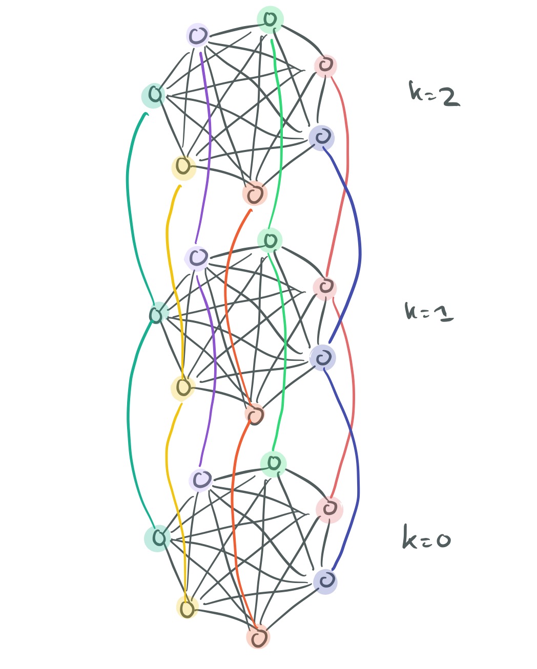
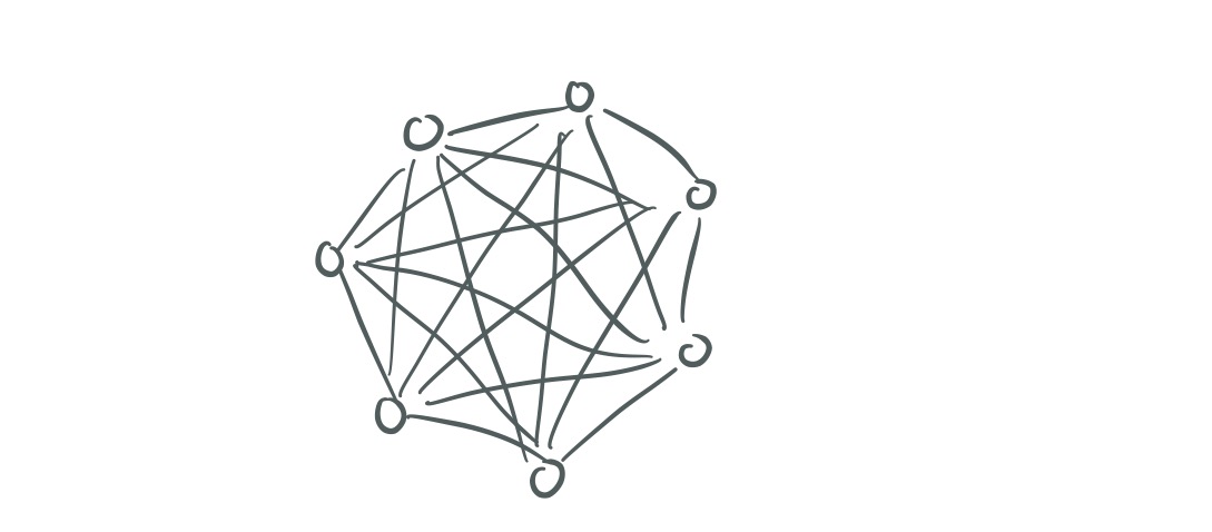
For a graph with diameter $k^{*}$ , we’re going to construct a multi-layer graph with $k^{*}$ levels. Each layer $k$ contains one node for each node in the original graph, and weighted undirected edges are created between the nodes in the layer according to their structural distance in their k-neighbourhood:
$w_{k}(uv,) = e^{-f_{k}(u,v)}$

Edges are defined only if $f_k(u,v)$ is defined. Here’s what one layer of the graph might look like.

Now we need to make connections across the layers. Each vertex is connected to its corresponding vertex in the layer above and the layer below. Moving down the layers, these edges simply have weight 1. Moving up the layers, the weight of the edge is based on the similarity $\Gamma_{k}(u)$ of a node $u$ to other nodes in layer $k$ .

$w(u_k,u_{k+1}) = \log(\Gamma_k(u) + e)$

$\Gamma_k(u)$ is the number of edges incident to $u$ that have weight larger than the average edge weight of the complete graph in layer $k$ .

Creating context through random walks

The context for a node $u$ is based on random walks in the multi-layer graph $M$ , starting at the corresponding vertex in layer 0. Repeating the walk a number of times yields multiple independent contexts for $u$ .

At each step in the random walk, we either move to another node in the current layer, or follow and edge to switch layers. The walk stays in the current layer with probability $q$ , choosing a node $v$ to walk to with probability

$p_{k}(u,v) = \frac{e^{-f_k(u,v)}}{Z_k(u)}$

Where $Z_k$ is just the normalization factor for the vertex $u$ in layer $k$ .

If we’re changing layers, then we go up a layer with probability proportional to the edge weight:

$p_k(u_k, u_{k+1}) = \frac{w(u_k, u_{k+1})}{w(u_k, u_{k+1}) + w(u_k, u_{k-1})}$

(And hence down a layer, if a lower layer exists, with probability $1 - p_k(u_k, u_{k+1})$ ).

Learning the vectors

Let the node sequences be generated by the random walks be the context, and use your favourite technique to learn a representation that predicts the context nodes for a given node $u$ . The authors used Skip-Gram for this.

Optimisations

In larger graphs, we can end up computing weights for a lot of edges ( $O(k^{*}n^3)$ ). To make the technique more practical the authors discuss three optimisations: reducing the length of degree sequences considered, reducing the number of pairwise similarity calculations, and reducing the number of layers. Details are in §3.5. The evaluation results show that this pragmatic pruning has only a small impact on the learned vectors’ effectiveness.

Evaluation

Barbell graphs

A Barbell graph is constructed with two complete graphs connected by a path graph, like so:

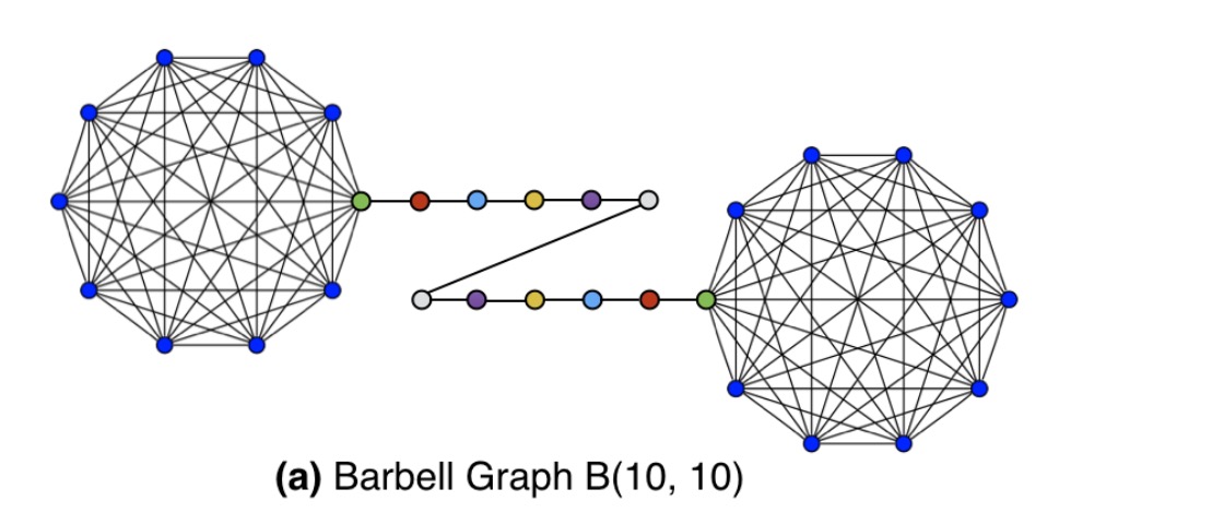
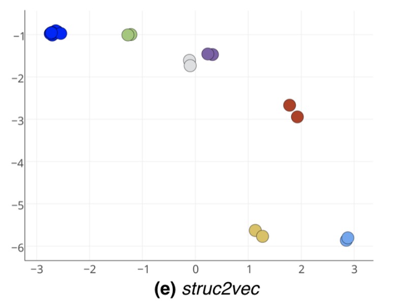
If we look at the latent node structure vectors learned by struc2vec, we see that all of the complete graphs nodes from both bells are clustered together (the blue dots), as are symmetrical points on the connecting path.

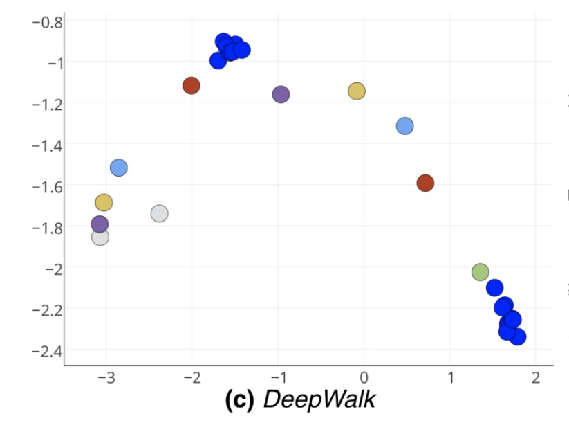
Other approaches, such as DeepWalk don’t cope so well with the structural similarity and e.g., create two different clusters of vectors for the two bells:

Karate Club network

The Karate Club network has 34 nodes and 78 edges, with each node representing a club member and an edge between members denoting that they have interacted outside of the club. The authors construct a network consisting of two identical copies of the Club network joined by one connecting edge:

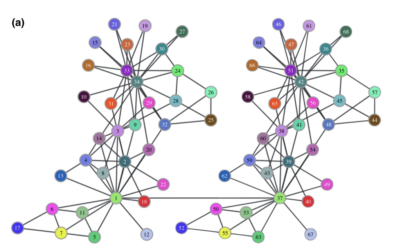
Struc2vec is able to closely pair the corresponding nodes in each half of the growth (which obviously have the same structure).

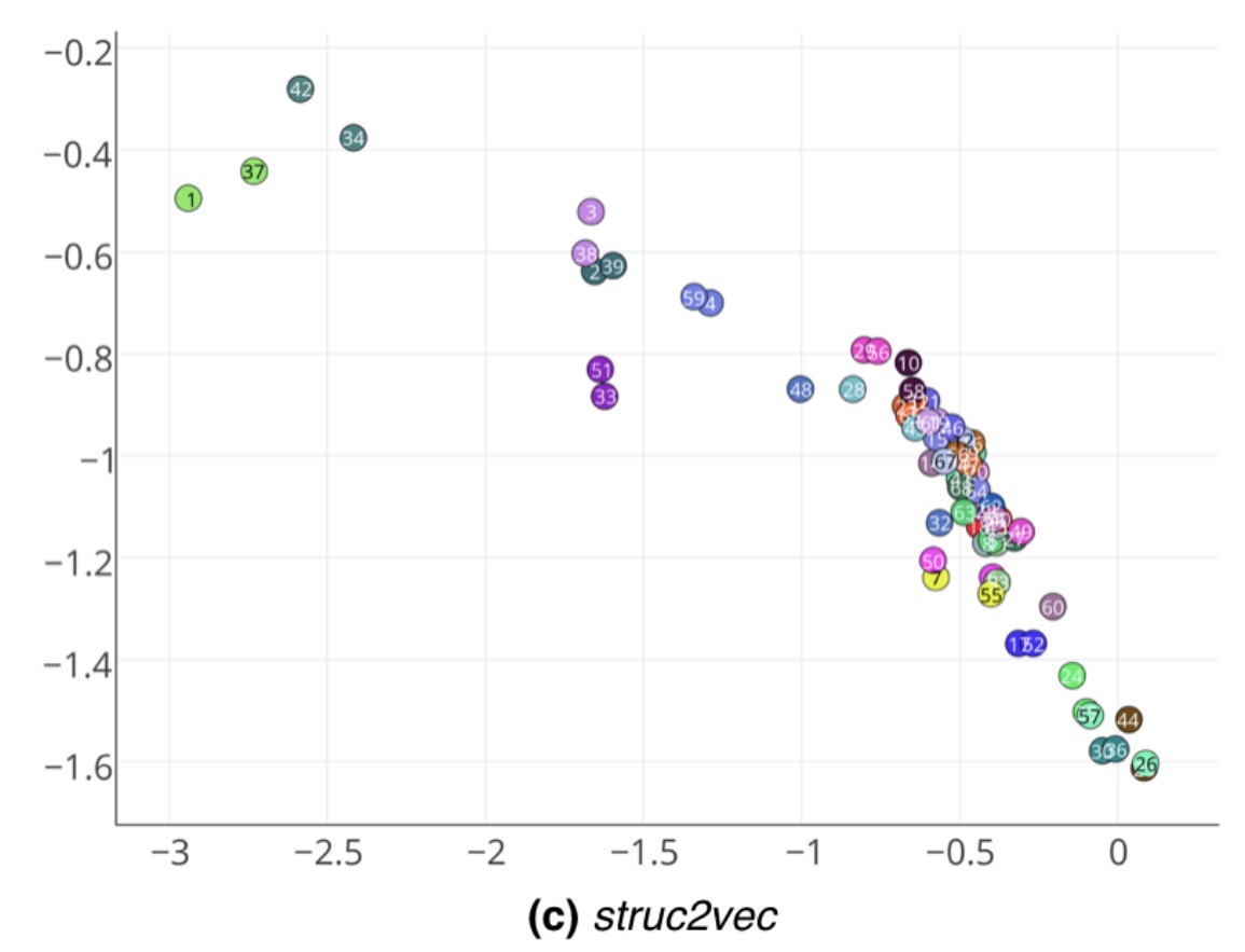
As an example, note that nodes 1, 34 and their correspondent mirrors (37 and 42) are in a separate cluster in the latent space. Interestingly, these are exactly the nodes that represent the club instructor Mr. Hi and his administrator John A. The network was gathered after a conflict between the two split the members of the club into two groups – centered on either Mr. Hi or John A. Therefore, nodes 1 and 34 have the specific and similar role of leaders in the network. Note that struc2vec captures their function even though there is no edge between them.

Robustness to noise

Starting with an egonet graph extracted from Facebook, edge sampling is used to create two new graphs in which each edge from the original graph is present with some probability $s$ . For varying values of s, the following chart shows the distance in latent space between corresponding node pairs and all node pairs. Even when s = 0.3, so that the probability that an original edge appears in both sampled graphs is 0.09 (0.3^2), the framework still places corresponding nodes closer in the latent space.

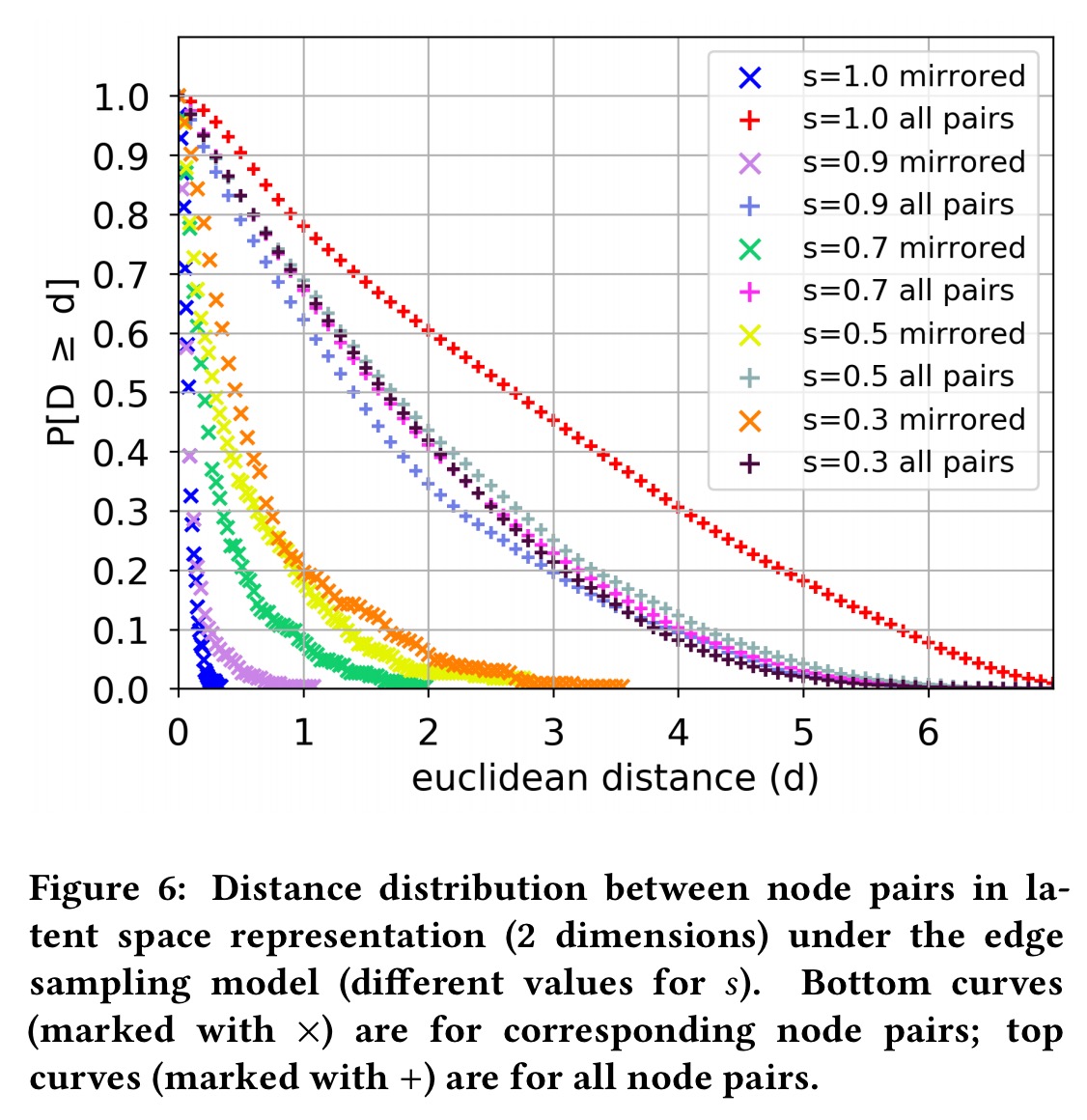
This experiment indicates the robustness of the framework in uncovering the structural identity of nodes even in the presence of structural noise, modeled here through edge removals.

Using the learned vectors for classification

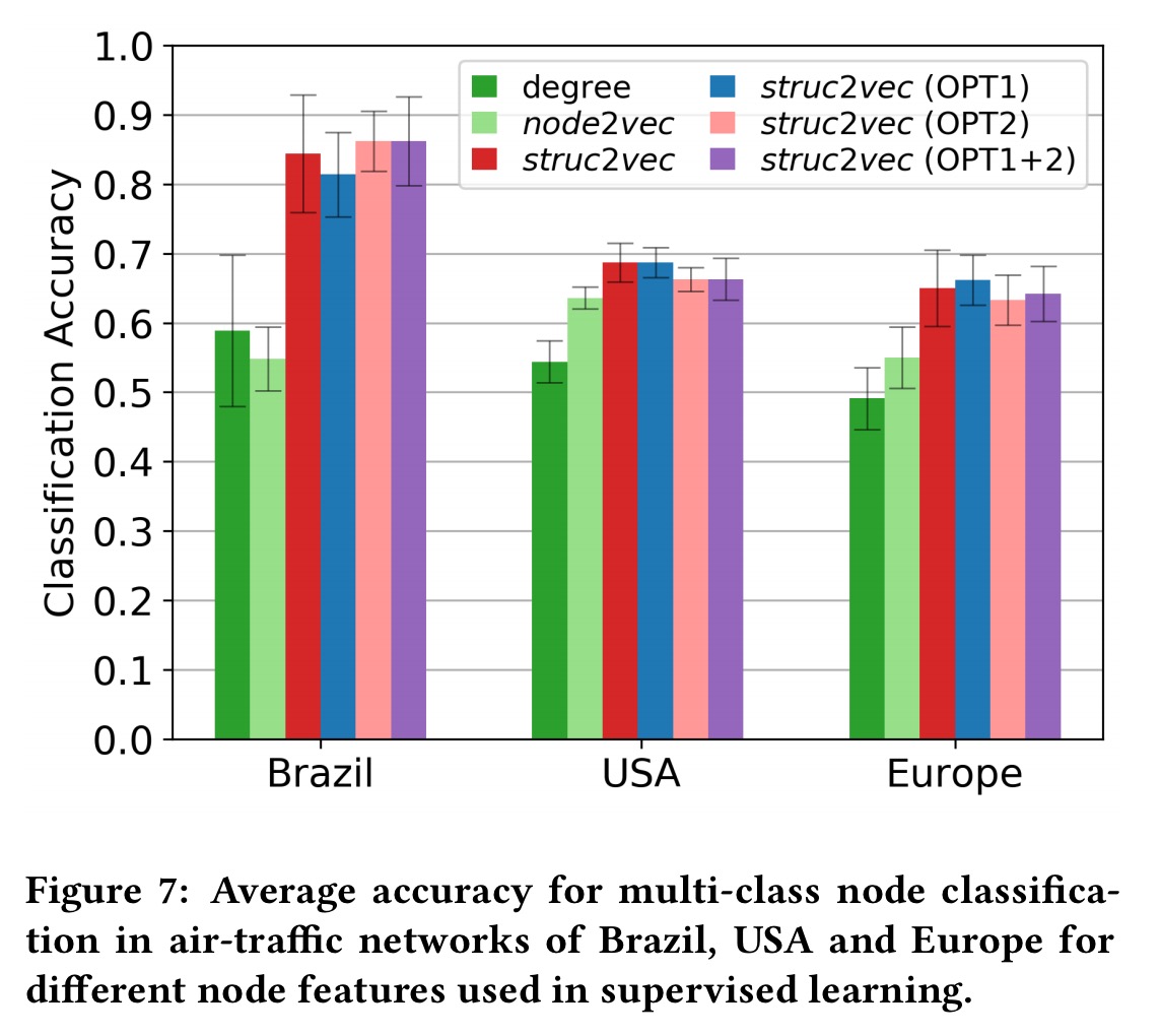
In a final experiment, the authors take air traffic network graphs for Brazil, America, and Europe where nodes correspond to airports and edges correspond to commercial flights. The struc2vec latent vectors are used to train a supervised classifier which predicts how active the airport is (which quartile the airport appears in when ranked by busyness). The struc2vec vectors are compared against alternative features for this task: simple node degree, and a prior work node2vec. Struc2vec demonstrates superior classification accuracy on this task.

the morning paper

a random walk through Computer Science research, by Adrian Colyer
Made delightfully fast by strattic