Statistical analysis of latency through semantic profiling Huang et al., EuroSys’17
Unlike traditional application profilers that seek to show the ‘hottest’ functions where an application spends the most time, VProfiler shows you where the sources of variance in latency come from, tied to semantic intervals such as individual requests or transactions.
… an increasing number of modern applications come with performance requirements that are hard to analyze with existing profilers. In particular, delivering predictable performance is becoming an increasingly important criterion for real-time or interactive applications, where the latency of individual requests is either mission-critical or affecting user experiences.
The authors used VProfiler to analyse MySQL, Postgres, and Apache Web Server, finding major sources of latency variance for transactions / web requests respectively. These are complex code bases that are hard to analyse by hand (e.g. MySQL has 1.5M lines of code and 30K functions).
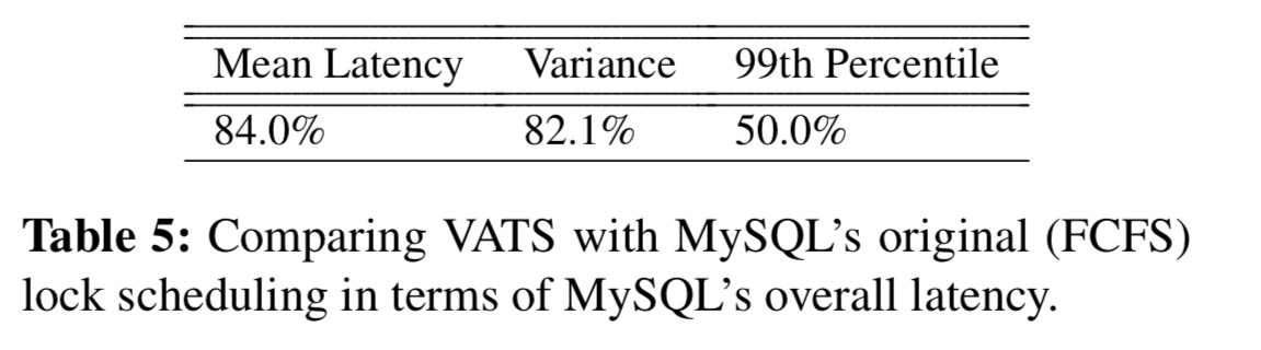
We show that VProfiler’s results are insightful and lead to application-specific optimizations that significantly reduce the overall mean, variance, and 99th percentile latencies by 84%, 82%, and 50% respectively.
The proposed change to MySQL that the team made after being pointed to the right place by VProfiler has been included in MySQL distributions and made the default behaviour in MariaDB from v10.2.3 onwards. So you might soon be benefiting from the work described in this paper even if you don’t use VProfiler yourself!
While the goal of VProfiler is to reduce latency variance (without increasing overall latency!), the changes pointed to by VProfiler also had the side-effect of reducing mean latency, coefficient of variation, and tail latency. (The coefficient of variation is the ratio of the standard deviation to the mean).
It all sounds very interesting indeed! Currently VProfiler only works with C/C++ code, but a Java version is in the works. If you want to play with it, you can find it on github here: https://github.com/mozafari/vprofiler (with thanks to Barzan Mozafari for the link).
Using VProfiler
The first step in using VProfiler is to annotate the target program using three annotations that identify: (i) when a new semantic interval is created (e.g., transaction start), (ii) when a semantic interval is complete (e.g., transaction commit), and (iii) when a thread begins executing on behalf of a specific semantic interval – for example, a worker thread dequeues and executes an event associated with the semantic interval. Note that the start and end events don’t have to be on the same thread – event driven architectures are fully supported.
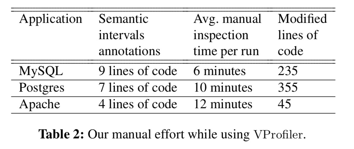
The annotation of semantic intervals requires only a few lines of code. We expect this to hold in most cases, as the notion of a semantic interval is typically intuitive to developers (e.g., a request or a transaction). Identifying the synchronization functions is similarly straightforward, as codebases typically use a well-defined API for synchronization.
Here are the details of lines changed in the three systems in the study:
VProfiler then instruments the code and an initial run is done using some suitable workload. VProfiler reports back to the developer the top-k factors (sources of variance) when profiling a subset of functions, starting at the root of the call graph. The subset of functions that are profiled is simply determined by call-graph depth.
This profile is then returned to the developer, who determines if the profile is sufficient. If not, the children of the top-k factors are added to the list of functions to be profiled, instrumentation code is automatically inserted by VProfiler, and a new profile is collected.
The process repeats iteratively until the developer is satisfied the information provided is of sufficient detail. Because the tree is only ever expanded in the regions of the top-k factors, the profiling overhead is kept low.
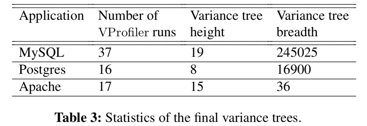
For MySQL, Postgres, and Apache, here are the number of profiler runs and ultimately profile tree (variance tree) size:
Determining execution variance using variance trees
Now we turn our attention to how VProfiler determines the top-k factors during a run. Everything starts with segments, which are contiguous time intervals on a single thread that are labelled as part of at most a single semantic interval.
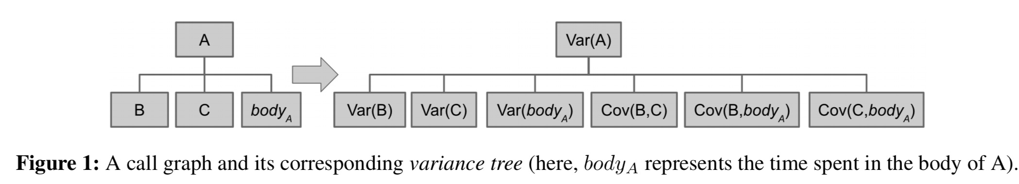
VProfiler analyzes performance variance by comparing the duration of particular function invocations in an executing segment across other invocations of the same function in different semantic intervals (i.e., it analyzes variances of invocations of the same function across different requests). VProfiler uses a novel abstraction, the variance tree, to reason about the relationship between latency variance and the call hierarchy rooted at a particular function invocation.
Within a segment, VProfiler tracks the variance of each function and the covariance of each pair of children in the call graph. This information forms a variance tree. It’s easiest to see by example: in the figure below we’re profiling a function A, which calls B and C as well as spending time in its own function body of course.
The variance tree enables quick detection of sub-trees that do not contribute to latency variability, but identifying the root causes of high variability is harder.
The variance of a parent node is always larger than any of its children, so simply identifying the nodes with the highest variance is not useful for understanding the cause of that variance. Furthermore, some variance arises because invocations may perform more work and manipulate more data (e.g., a transaction accessing more records).
We’re not interested in the second kind of variance. The high-level goal is to identify functions (or co-varying function pairs) that (1) account for a substantial fraction of overall latency variance and (2) can reveal insights as to why variance occurs. The variance of a function, or the co-variance of a function pair, are both described as factors.
Our intuition is that functions deeper in the call graph implement narrower and more specific functionality, hence, they are more likely to reveal the root cause of latency variance.
If A calls B and C, and A accounts for 30% of transaction variance overall, but within A, B accounts for 28% of variance, then B is likely to be more informative than A.
VProfiler therefore ranks factors using a scoring function that considers both the magnitude of the variance attributed to the factor, and its height (maximum depth of the call tree beneath it).
The specificity of a factor is the square of the difference in height between the root of the call graph within the segment, and the height of the factor under consideration. So, e.g., a factor with height 4 in an overall call graph of height 7 will have a specificity score of 9. The overall scoring function simply multiplies the specificity by the factor’s variance (or covariance, as applicable).
The scoring and ranking takes place in an offline analysis phase after a run is complete. VProfiler works backwards from the final segment of a semantic interval, aggregating latency and variance of preceding functions on the same thread until it encounters an incoming wake-up edge indicating execution on this segment was triggered by an event elsewhere. It will then follow this edge, performing aggregation along the target thread, and so on.
Intuitively, we conceive of VProfiler as assigning “blame” for accumulated delay leading to the completion of a semantic interval; blame propagates backwards along segments and their dependencies.
In the workloads studied by the authors pre-emption is rare as the thread pool sized is tuned not to exceed the number of available cores, so there was no need to instrument the OS scheduler.
Case studies
… we conduct case studies on three popular open-source systems: MySQL (a thread-per-connection database), Postgres (a process-per-connection database), and Apache Web Server (an event-based server application). For MySQL and Postgres, we treat each ‘transaction’ as a semantic interval, while for Apache we treat each ‘web request’ as a semantic interval.
MySQL is tested using the TCP-C benchmark in two configurations: one with 128 Warehouses, and one with 2 (128-WH and 2-WH). The major sources of variance are shown in the following table:
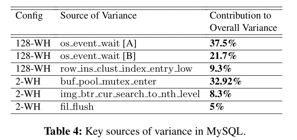
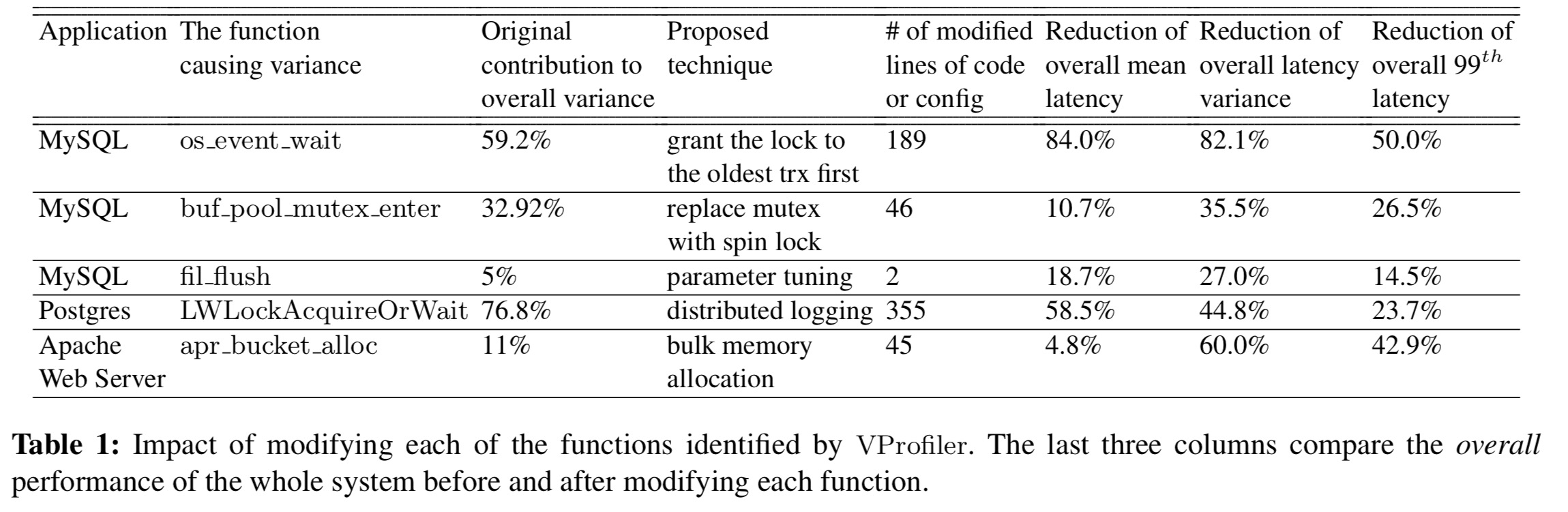
The next step is of course manual inspection of these functions to understand why. As an example, the os_event_wait A and B entries refer to the two most important call sites for os_event_wait which correspond to locks acquired during select and update statements respectively.
The high variance of these call sites reflects the high variability in the wait time for contended locks, which contributes to more than half of the overall latency variance. Our fix is to replace MySQL’s lock scheduling strategy, which is based on First Come First Served (FCFS), with a Variance-Aware-Transaction-Scheduling (VATS) strategy that minimizes overall wait time variance. In short, VATS uses an Oldest Transaction First (grant the lock to the oldest transaction) strategy as an alternative to FCFS. As shown in Table 5, VATS reduces 82.1% of the overall latency variance and 50.0% of the 99th percentile latency (for
the TPC-C workload).
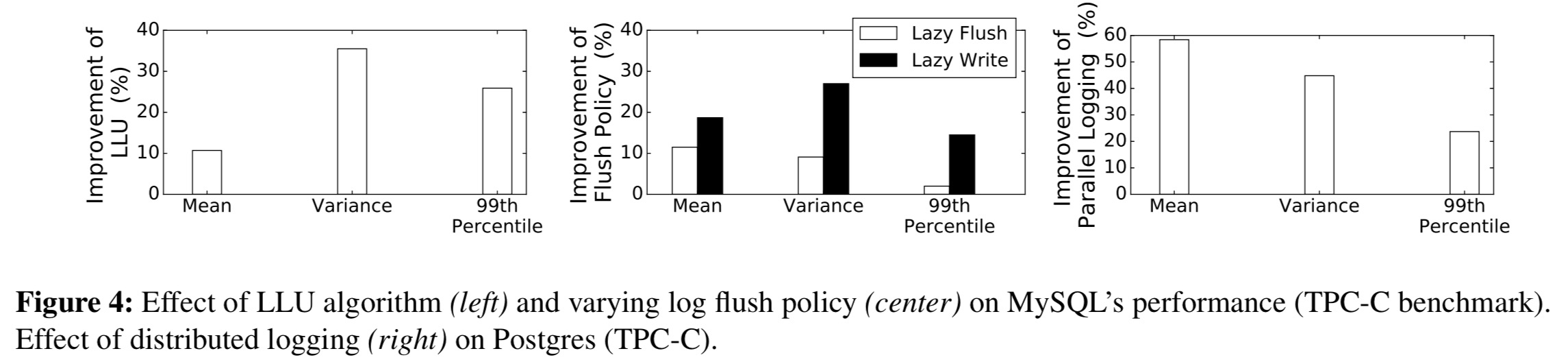
In the 2-WH configuration, an analysis of buf_pool_mutex_enter identifies waiting on a global lock for the buffer page list as the chief culprit. Changing the code to abort a page moving operation if the lock is not granted in time, and retry the next time the lock is successfully acquired (Lazy LRU Update, LLU) eliminated 35.5% of the overall variance.
Some of the other functions reported by the profiler showed variance inherent to the transactions rather than performance pathologies and so no action needed to be taken there.
Postgres is investigated using a 32-warehouse TPC-C configuration, resulting in the following key sources of variance:
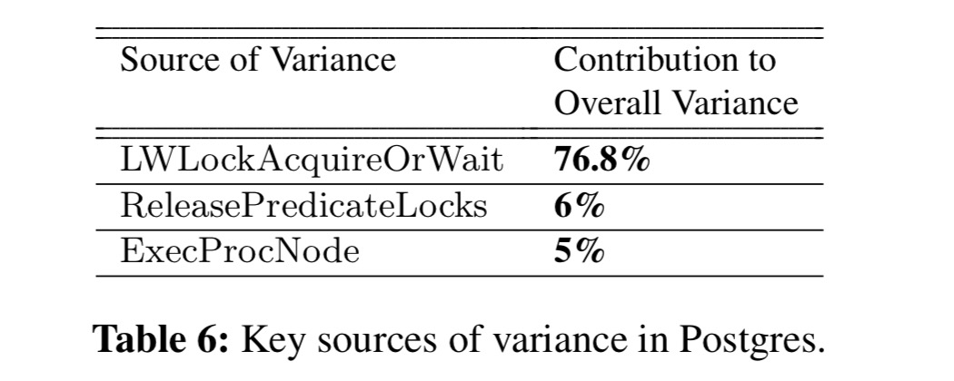
In LWLockAcquireOrWait Postgres acquires an exclusive lock to protect the redo log and ensure only one transaction at a time can write to it. The authors tested an approach to reducing contention that involved using two separate hard disks for storing two sets of redo logs. A transaction then only needs to wait when neither set is available. This eliminates 58.5% of the overall mean latency.
The improvements across MySQL and Postgres from the three changes we have discussed so far can be seen in the following figure:
Apache was tested using ApacheBench simulating 1000 clients making 20000 requests. The top factors here were all co-variances:
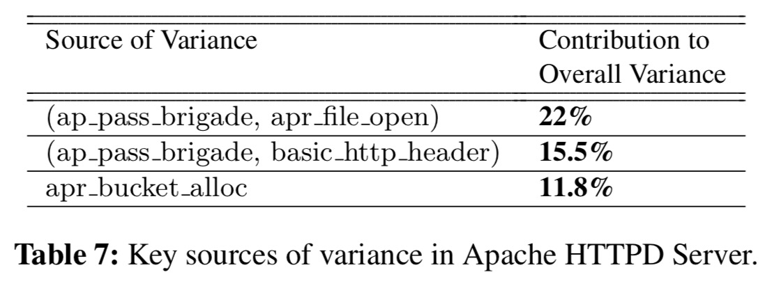
On investigation, these all turned out to be memory-allocation related. Modifying the memory management library to pre-allocate larger chunks of memory in advance eliminated 60% of the overall variance in Apache request latencies.
Here’s a summary of the main changes that VProfiler led the authors to and their impact, across all three systems in the study:

Very useful. Thanks for raising awareness.