DeepSense: a unified deep learning framework for time-series mobile sensing data processing Yao et al., WWW’17

DeepSense is a deep learning framework that runs on mobile devices, and can be used for regression and classification tasks based on data coming from mobile sensors (e.g., motion sensors). An example of a classification task is heterogeneous human activity recognition (HHAR) – detecting which activity someone might be engaged in (walking, biking, standing, and so on) based on motion sensor measurements. Another example is biometric motion analysis where a user must be identified from their gait. An example of a regression task is tracking the location of a car using acceleration measurements to infer position.

Compared to the state-of-art, DeepSense provides an estimator with far smaller tracking error on the car tracking problem, and outperforms state-of-the-art algorithms on the HHAR and biometric user identification tasks by a large margin.

Despite a general shift towards remote cloud processing for a range of mobile applications, we argue that it is intrinsically desirable that heavy sensing tasks be carried out locally on-device, due to the usually tight latency requirements, and the prohibitively large data transmission requirement as dictated by the high sensor sampling frequency (e.g., accelerometer, gyroscope). Therefore we also demonstrate the feasibility of implementing and deploying DeepSense on mobile devices by showing its moderate energy consumption and low overhead for all three tasks on two different types of smart device.

I’d add that on-device processing is also an important component of privacy for many potential applications.

In working through this paper, I ended up with quite a few sketches in my notebook before I reached a proper understanding of how DeepSense works. In this write-up I’m going to focus on taking you through the core network design, and if that piques your interest, the rest of the evaluation details etcetera should then be easy to pick up from the paper itself.

Processing the data from a single sensor

Let’s start off by considering a single sensor (ultimately we want to build applications that combine data from multiple sensors). The sensor may provide multi-dimensional measurements. For example, a motion sensor that report motion along , and axes. We collect sensor readings in each of these dimensions at regular intervals (i.e., a time series), which we can represent in matrix form as follows:

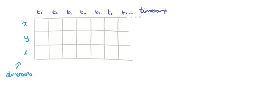
We’re going to process the data in non-overlapping windows of width . Dividing the number of data points in the time series sample by gives us the total number of windows, . For example, if we have 5 seconds of motion sensor data and we divide it into windows lasting 0.25s each, we’ll have 20 windows.

Finding patterns in the time series data works better in the frequency dimension than in the time dimension, so the next step is to take each of the windows, and pass them through a Fourier transform resulting in frequency components, each with a magnitude and phase. This gives us a matrix for each window.

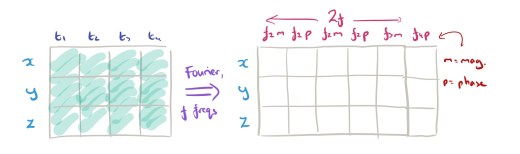
We’ve got of these, and we can pack all of that data into a tensor.

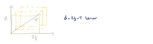
It’s handy for the implementation to have everything nicely wrapped up in a single tensor at this point, but actually we’re going to process slice by slice in the dimension (one window at a time). Each window slice is passed through a convolution neural network component comprising three stages as illustrated below:

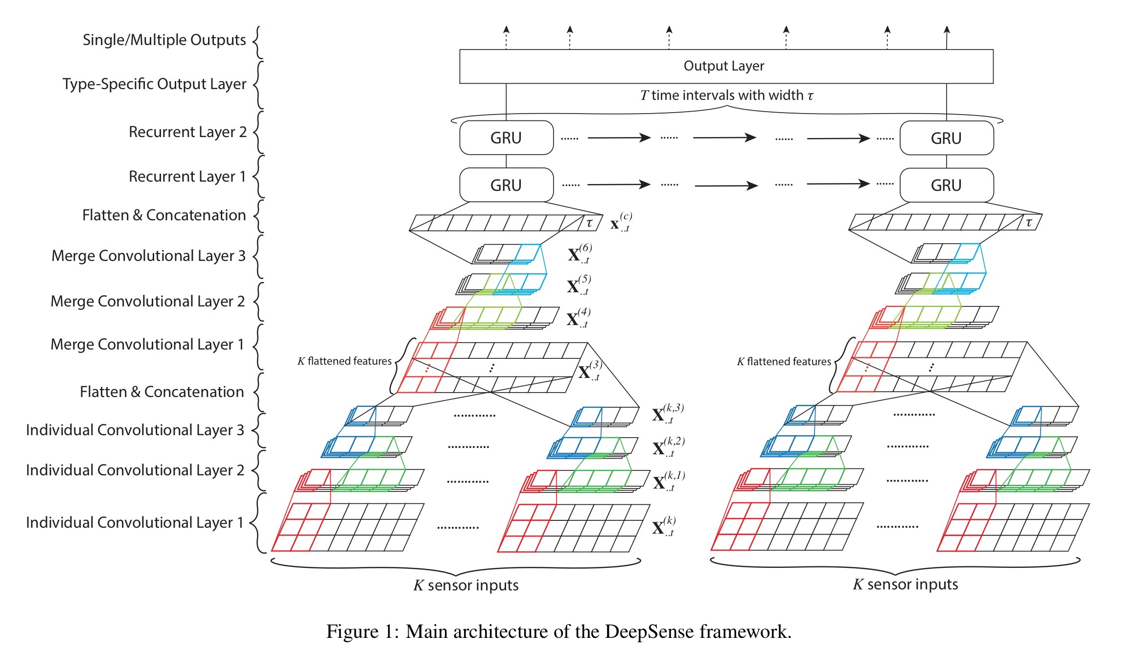
First we use 2D convolutional filters to capture interactions among dimensions, and in the local frequency domain. The output is then passed through 1D convolutional filter layers to capture high-level relationships. The output of the last filter layer is flatten to yield sensor feature vector.

Combining data from multiple sensors

Follow the above process for each of the sensors that are used by the application. We now have sensor feature vectors, that we can pack into a matrix with rows.

The sensor feature matrix is then fed through a second convolutional neural network component with the same structure as the one we just looked at. That is, a 2D convolutional filter layer followed by two 1D layers. Again, we take the output of the last filter layer and flatten it into a combined sensors feature vector. The window width is tacked onto the end of this vector.

For each convolutional layer, DeepSenses learns 64 filters, and uses ReLU as the activation function. In addition, batch normalization is applied at each layer to reduce internal covariate shift.

Now we have a combined sensors feature vector for one time window. Repeat the above process for all T windows.

Use an RNN to learn patterns across time windows

So now we have combined sensor feature vectors, each learning intra-window interactions. But of course it’s also important to learn inter-window relationships across time windows. To do this the feature vectors are fed into an RNN.

At this point I think we’re ready for the big picture.

Instead of using LSTMs, the authors choose to use Gated Recurrent Units (GRUs) for the RNN layer.

… GRUs show similar performance to LSTMs on various tasks, while having a more concise expression, which reduces network complexity for mobile applications.

DeepSense uses a stacked GRU structure with two layers. These can run incrementally when there is a new time window, resulting in faster processing of stream data.

Top it all with an output layer

The output of the recurrent layer is a series of vectors, , one for each time window.

For regression-based tasks (e.g., predicting car location), the output layer is a fully connected layer on top of each of those vectors, sharing weights and bias term to learn .

For classification tasks, the individual vector are composed into a single fixed-length vector for further processing. You could use something fancy like a weighted average over time learned by an attention network, but in this paper excellent results are obtained simply by averaging over time (adding up the vectors and dividing by ). This final feature vector is fed into a softmax layer to generate the final category prediction.

Customise for the application in hand

To tailor DeepSense for a particular mobile sensing and computing task, the following steps are taken:

• Identify the number of sensor inputs, , and pre-process the inputs into a set of tensors.
• Identify the type of the task and select the appropriate output layer
• Optionally customise the cost function. The default cost function for regression oriented tasks is mean squared error, and for classification it is cross-entropy error.

For the activity recognition (HHAR) and user identification tasks in the evaluation the default cost function is used. For car location tracking a negative log likelihood function is used (see section 4.2 for details).

Key results

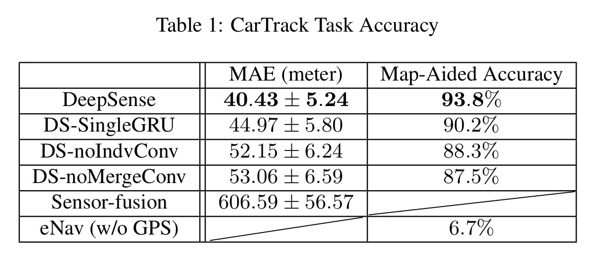
Here’s the accuracy that DeepSense achieves on the car tracking task, versus the sensor-fusion and eNav algorithms. The map-aided accuracy column shows the accuracy achieved when the location is mapped to the nearest road segment on a map.

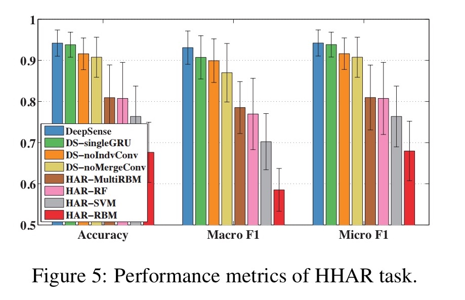
On the HHAR task DeepSense outperforms other methods by 10%.

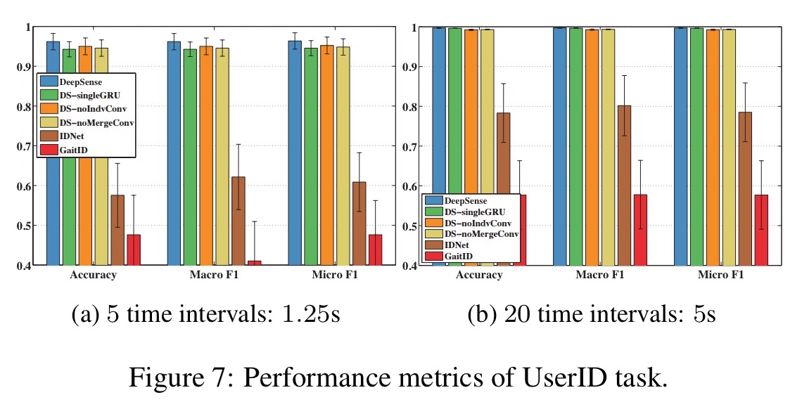
And on the user identification task by 20%:

We evaluated DeepSense via three representative mobile sensing tasks, where DeepSense outperformed state of the art baselines by significant margins while still claiming its mobile-feasibility through moderate energy consumption and low latency on both mobile and embedded platforms.

The evaluation tasks focused mostly on motion sensors, but the approach can be applied to many other sensor types including microphone, Wi-Fi signal, Barometer, and light-sensors.