Trajectory recovery from Ash: User privacy is NOT preserved in aggregated mobility data Xu et al., WWW’17

Borrowing a little from Simon Wardley’s marvellous Enterprise IT Adoption Cycle, here’s roughly how my understanding progressed as I read through this paper:

Huh? What? How? Nooooo, Oh No, Oh s*@\#!

Xu et al. show us that even in a dataset in which you might initially think there is no chance of leaking information about individuals, they can recover data about individual users with between 73% and 91% accuracy. Even in datasets which aggregate data on tens of thousands to hundreds of thousands of users! Their particular context is mobile location data, but underpinning the discovery mechanism is a reliance on two key characteristics:

1. Individuals tend to do the same things over and over (regularity) – i.e., there are patterns in the data relating to given individuals, and
2. These patterns are different across different users (uniqueness).

Therefore, statistical data with similar features is likely to suffer from the same privacy breach. Unfortunately, these two features are quite common in the traces left by humans, which have been reported in numerous scenarios, such as credit card records, mobile application usage, and even web browsing. Hence, such a privacy problem is potentially severe and universal, which calls for immediate attention from both academia and industry.

(Emphasis mine). As we’ll see, there are a few other details that matter which in my mind might make it harder to transfer to other problem domains – chiefly the ability to define appropriate cost functions – but even if it does relate only to location-based data, it’s still a very big deal.

Let’s take a look at what’s in a typical aggregated mobility dataset, and then go on to see how Xu et al. managed to blow it wide open.

Aggregated mobility data (ash)

In an attempt to preserve user privacy, owners of mobility data tend to publish only aggregated data, for example, the number of users covered by a cellular tower at a particular timestamp. The statistical data is of broad interest with applications in epidemic controlling, transportation scheduling, business intelligence, and more. The aggregated data is sometimes called the ash of the original trajectories.

The operators believe that such aggregation will preserve users’ privacy while providing useful statistical information for academic research and commercial usage.

To publish aggregated mobility data, first the original mobility records of individual mobile users are grouped by time slots (windows), then for each window, aggregate statistics are computed (e.g., the number of mobile users covered by each base station).

Two desirable properties are assumed to hold from following such a process:

1. No individual information can be directly acquired from the datasets, with the aggregated mobility data complying with the k-anonymity privacy model.
2. The aggregate statistics are accurate.

Although the privacy leakage in publishing anonymized individual’s mobility records has been recognized and extensively studied, the privacy issue in releasing aggregated mobility data remains unknown.

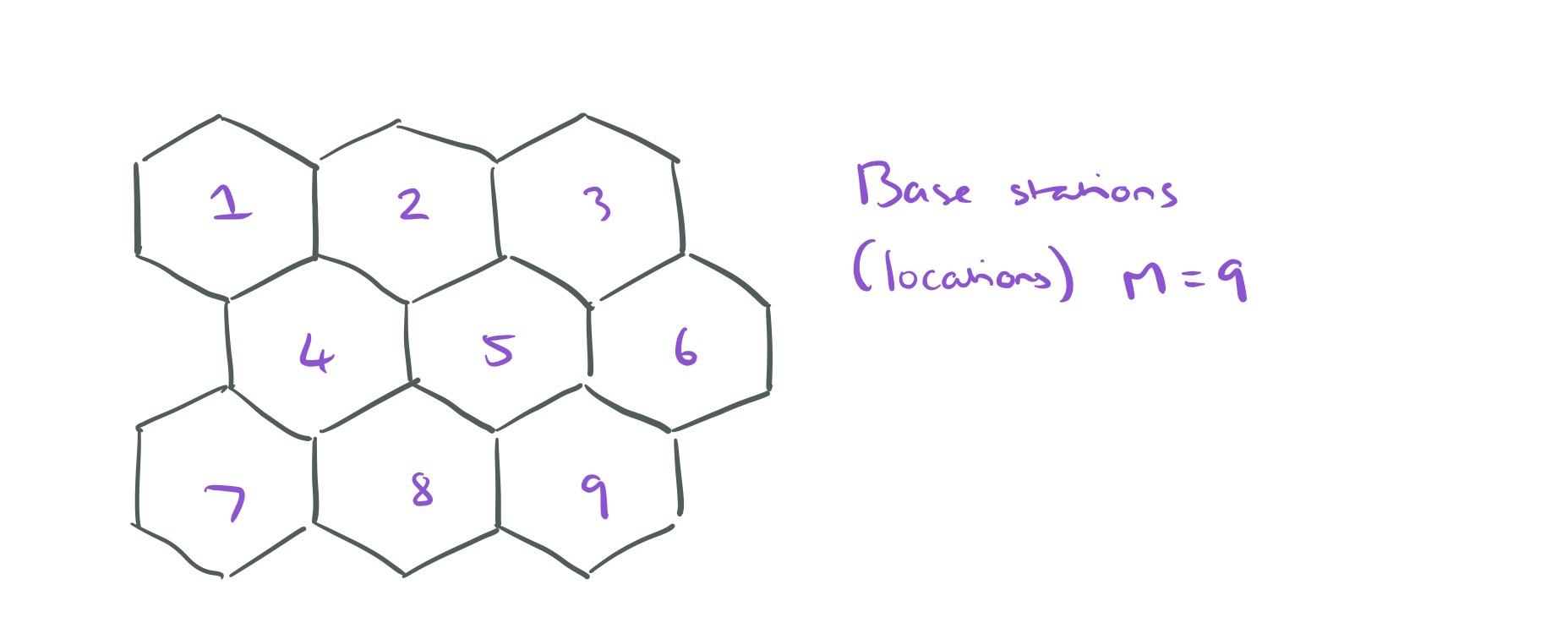
Looking at this from a differential privacy perspective, you might already be wondering about the robustness of being able to detect e.g., whether or not a particular individual is represented in the dataset. But what we’re about to do goes much further. Take a dataset collected over some time period, which covers a total of M locations (places). In each time slot, we have the number of users in each of those places (i.e., an M-dimensional vector). That’s all you get. From this information only, it’s possible to recover between 73% – 91% of all the individual users’ trajectories – i.e., which locations they were in at which times, and hence how they moved between them.

Huh? What? How?

Revealing individual users from aggregate data

The first thing it’s easy to work out is how many individual users there are at any point in time, just sum up all of the user counts for each place at that time. Call that N.

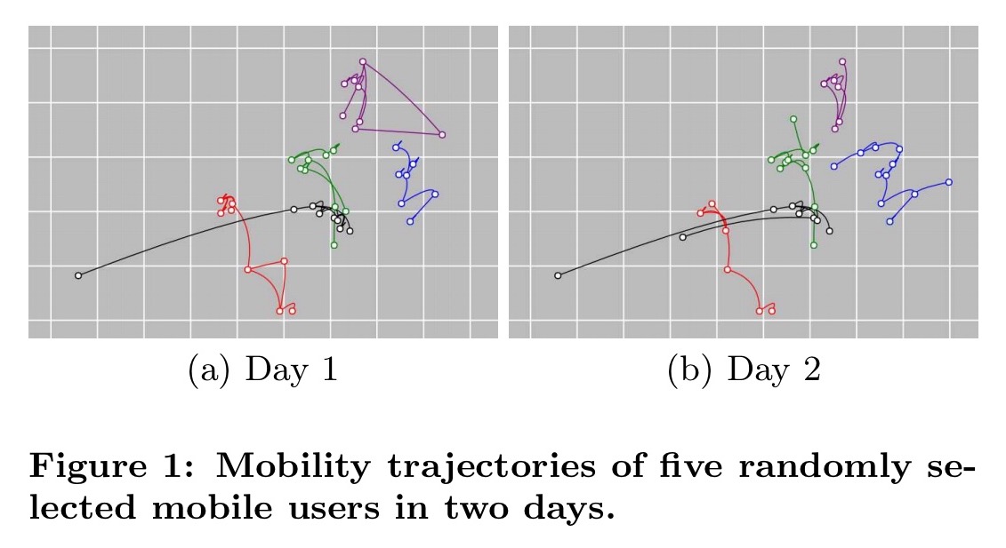
Now we need to consider what other clues might be available in the data. Individual users tend to have fairly coherent mobility trajectories (what they do today, they’re likely to do again tomorrow), and these trajectories are different across different users. See for example the trajectories of five randomly selected selected users over two days in the figure below. Each users’ pattern is unique, with strong similarity across both days.

The key to recovering individual trajectories is to exploit these twin characteristics of regularity for individual users, and uniques across users. Even so, it seems a stretch when all we’ve got is user counts by time and place!

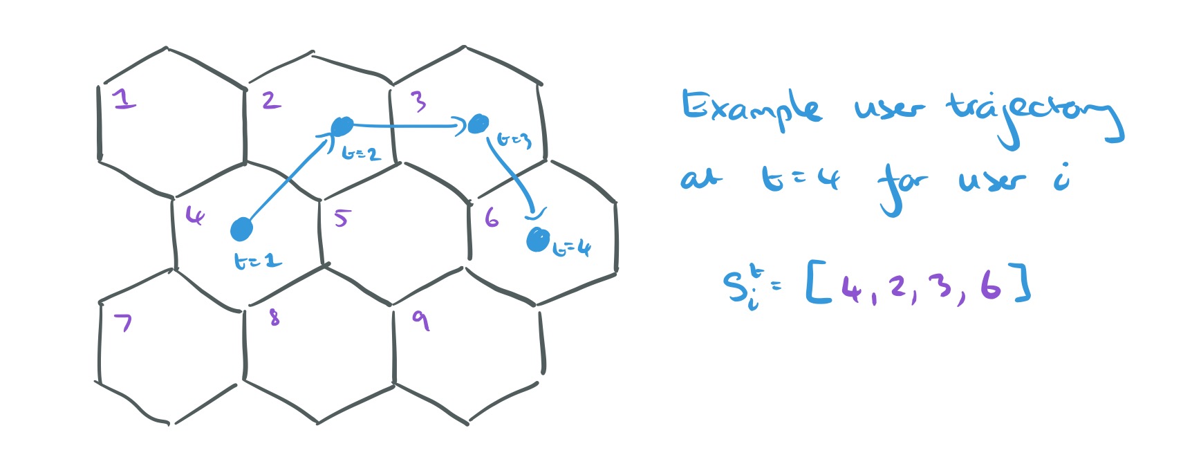
We’re going to build up estimates for the trajectories of each of the N users, one time step at a time. Let the estimate for the trajectory of the th individual user at time step t , be represented by a sequence of locations . For example, here’s a world with M=9 locations:

And here’s a trajectory for a user to time t, represented as a sequence of t locations:

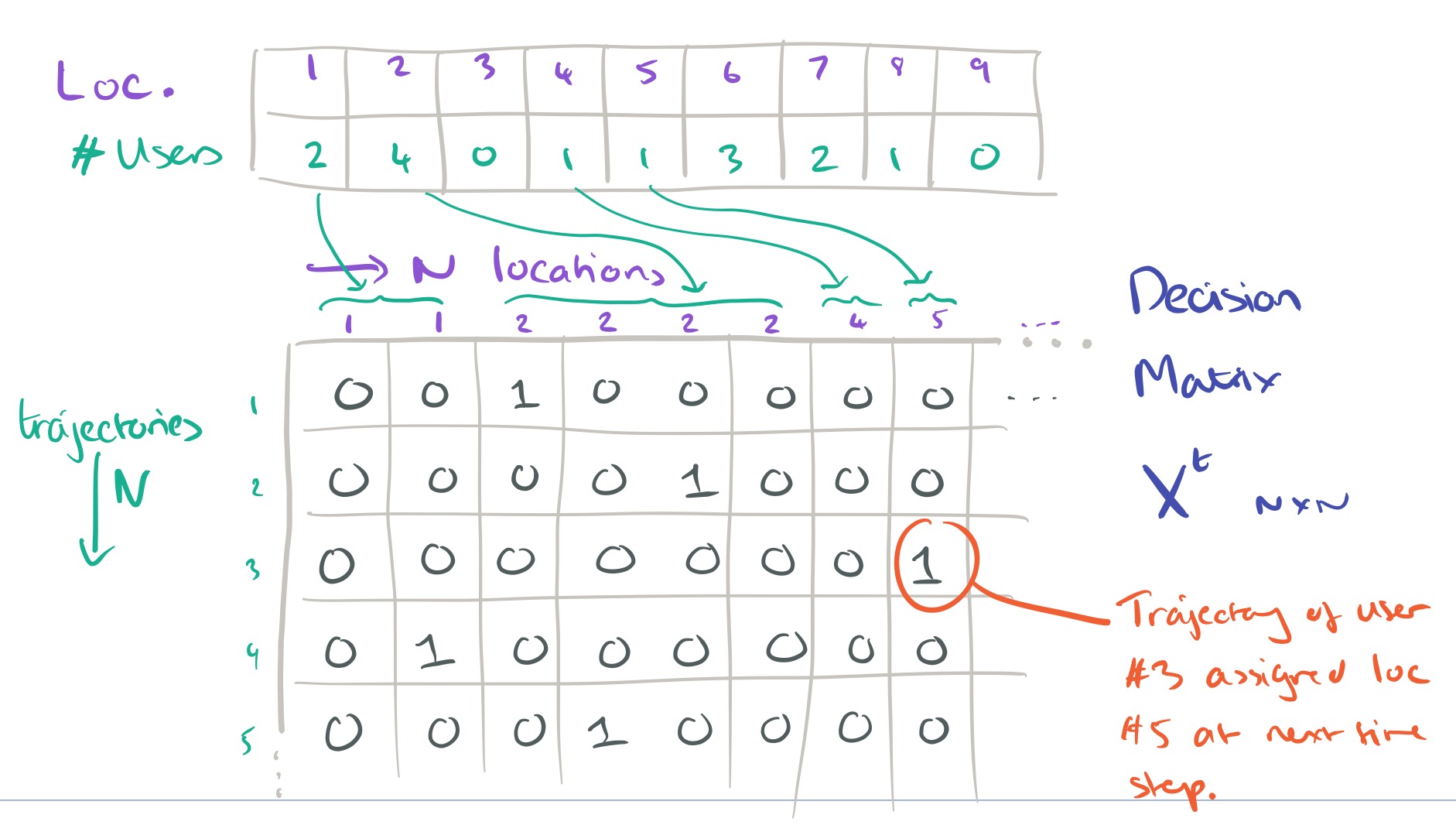
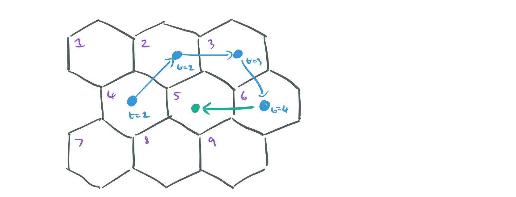
We want to decide on the most likely location for each user at time step t+1, subject to the overall constraint that we know how many users in total there must be at each location at time t+1. The description of how this next part works is very terse in the paper itself, but with a little bit of reverse engineering on my part I believe I’ve reached an understanding. The secret is to formulate the problem as one of completing a decision matrix. This decision matrix takes a special form, it has N rows (one for each user trajectory to date), and N columns. Say we know that there must be two users in location 1, and four users in location 2. Then the first two columns in the matrix will represent the two ‘slots’ available in location 1, and the next four columns will represent the four slots available in location 2, and so on.

In the decision matrix , if next location for trajectory is the location identified by column , and zero otherwise. A valid completion of the matrix has every row adding up to one (each trajectory is assigned one and only one next location), and every column adding up to one (each slot is filled by one and only one user).

Thus the example decision matrix above indicates that the next location for the trajectory of user #3 has been assigned as location 5.

When we complete the decision matrix, we don’t just make random assignments of slots of course! That’s where the cost matrix comes in. The cost matrix is also an NxN matrix, with the same row and column structure as the decision matrix. Instead of being filled with 1’s and 0’s though, contains a value representing the cost of moving to the location for slot given the trajectory so far for user . Take for example the trajectory for a user in the illustration below, which currently finishes in location 6. We might use as the cost of moving to each potential next location simply the number of hops in the grid to get there (red numbers). The actual cost functions used are more complex than this, this example is just to help you get the idea.

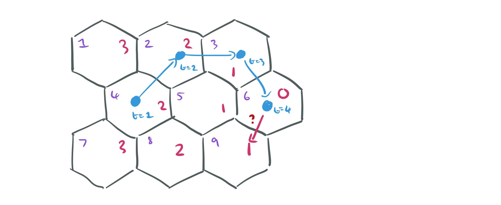
Here then is what a subsection of the cost matrix for the user in the above sketch might look like:

We’ll return to to how to define the cost functions in a moment. For now note that the problem has now become the following:

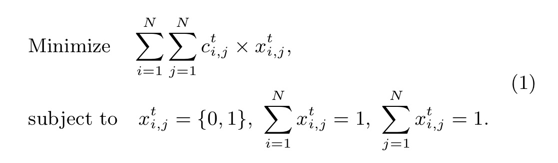
The above formulated problem is equivalent to the Linear Sum Assignment Problem, which has been extensively studied and can be solved in polynomial time with the Hungarian algorithm.

Space prevents me from explaining the Hungarian algorithm, but the Wikipedia link above does a pretty good job of it (it’s actually pretty straightforward, check out the section on the ‘Matrix interpretation’ to see how it maps in our case).

Thus far then, we’ve discovered a way to represent the problem such that we can recover each step of individual trajectories in polynomial time, so long as we can define suitable cost matrices.

Noooooo.

Building cost matrices – it’s night and day

At night time, people tend not to move around very much, as illustrated by these plots from two different datasets (the ‘operator’ dataset and the ‘app’ dataset) used in the evaluation:

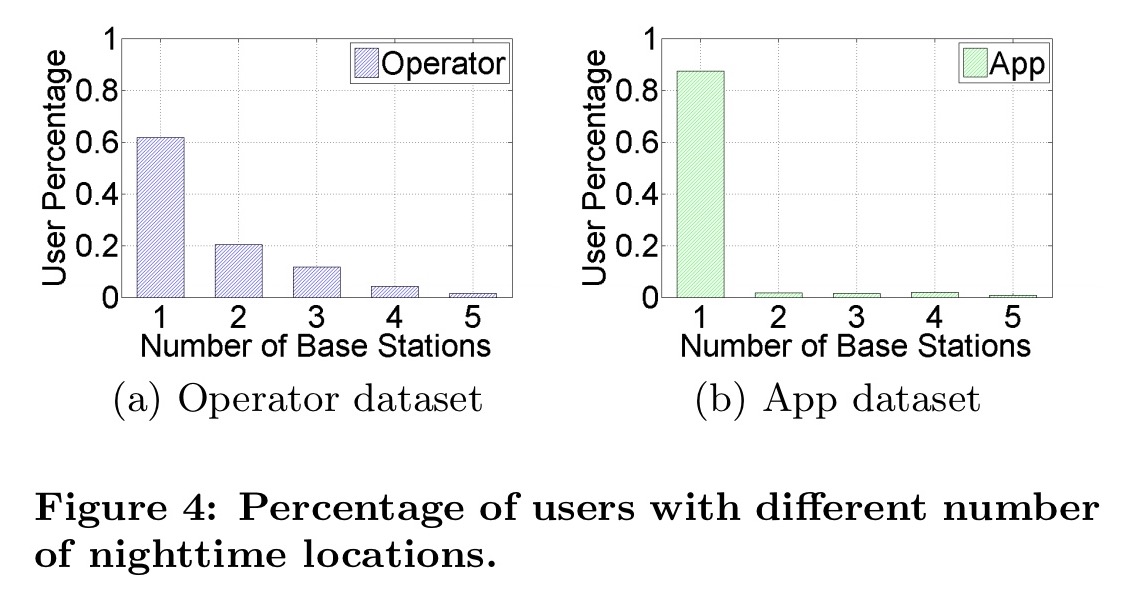
Not only that, but the night time location of individual users tends to be one of their top most visited locations (often the top location):

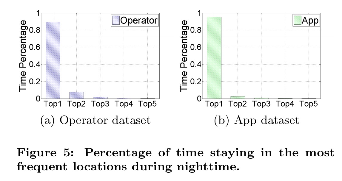
For the night time then, it makes sense to use the distance between the location of the user trajectory at time t and the location being considered for time t+1 as the cost.

In the daytime, people tend to move about.

The key insight is the continuity of human mobility, which enables the estimation of next location using the current location and velocity.

Let the estimated next location using this process be , then we can use as the cost function the distance between the and the location being considered for time t+1.

It is worth noting that the Hungarian algorithm is currently the most efficient algorithm to solve [the linear sum assignment problem], but still has computational complexity of . To speed things up, we adopt a suboptimal solution to reduce the dimension of the cost matrix by taking out the pairs of trajectories and location points with cost below a predefined threshold and directly linking them together.

Linking trajectories across days

Using the night and day approaches, we can recover mobile users’ sub-trajectories for each day. Now we need to link sub-trajectories together across days. Here we exploit the regularity exhibited in the day-after-day movements of individual users.

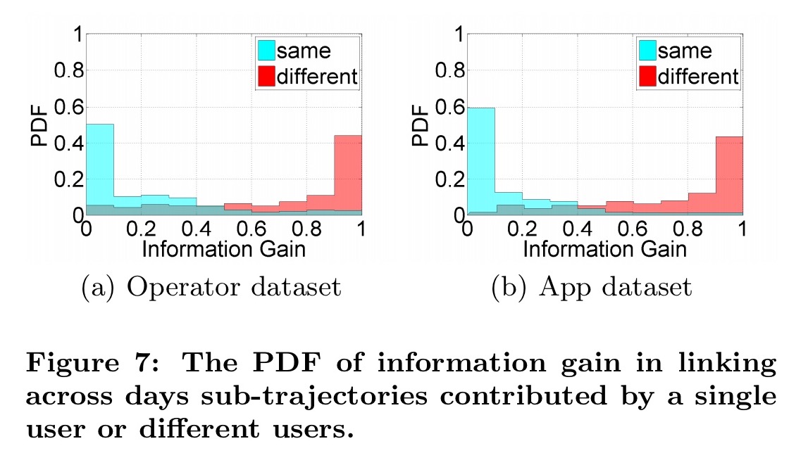
Specifically, we use the information gain of connecting two sub-trajectories to measure their similarities.

The entropy in a trajectory is modelled based on the frequency of visiting different locations, and the information gain from linking two sub-trajectories is modelled as the difference between the entropy of the combined trajectory, and the sum of the entropies of the individual trajectories over two. For the same user, we should see relatively little information gain if the two trajectories are similar, whereas for different users we should see much larger information gain. And indeed we do:

To conclude, we design an unsupervised attack framework that utilizes the universal characteristics of human mobility to recover individuals’ trajectories in aggregated mobility datasets. Since the proposed framework does not require any prior information of the target datasets, it can be easily applied on other aggregated mobility datasets.

Once the individual trajectories are separated out, it has been shown to be comparatively easy, with the help of small amounts of external data such as credit card records, to re-identify individual users (associated them with trajectories).

Oh no.

Evaluation

The authors evaluate the technique on two real world datasets. The ‘app’ dataset contains data for 15,000 users collected by a mobile app which records a mobile user’s location when activated, over a two-week period. The ‘operator’ dataset contains data for 100,000 mobile users from a major mobile network operator, over a one week period. Tests are run on aggregate data produced from these datasets, and the recovered trajectories are compared against ground truth.

In the figures that follow, stage #1 represents night time trajectory recovery, stage #2 day time trajectory recovery, and stage #3 the linking of sub-trajectories across days. Here we can see the recovery accuracy for the two datasets:

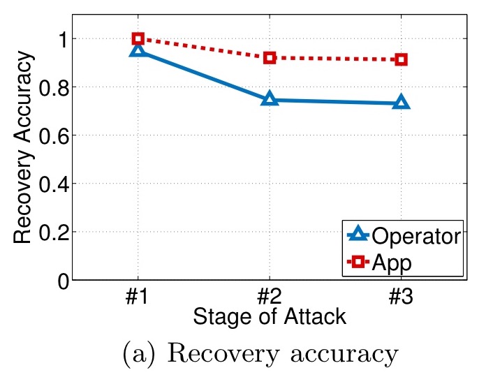
For the app dataset, 98% of night time trajectories are correctly recovered, failing to 91% accuracy by the final step. The corresponding figures for the operator dataset are 95% and 73%.

For the recovered trajectories, the following chart shows the percentage that can be uniquely identified given just the top-k locations for k=1 to 5.

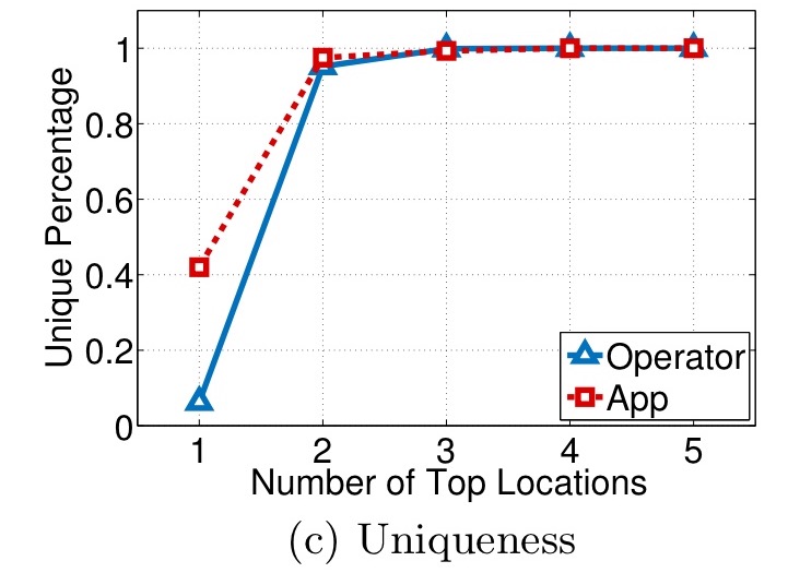
From the results, we can observe that given the two most frequent locations of the recovered trajectories, over 95% of them can be uniquely distinguished. Therefore, the results indicate that the recovered trajectories are very unique and vulnerable to be reidentified with little external information.

To put that more plainly, given the aggregated dataset, and knowledge of your home and work locations, there’s a very good chance I can recover your full movements!!!

Oh s*@\#!

Decreasing the spatial resolution (i.e., using more coarse-grained locations) actually increases the chances of successful trajectory recovery (but only to the location granularity of course). It’s harder to link these recovered trajectories to individual people though as human mobility becomes less unique in coarser-grained datasets.

Decreasing the temporal resolution (only releasing data for larger time windows) increases both the chances of successful trajectory recovery, and of re-identification.

The best defence for preserving privacy in aggregated mobility datasets should come as no surprise to you – we need to add some carefully designed random noise. What that careful design is though, we’re not told!

… a well designed perturbation scheme can reduce the regularity and uniqueness of mobile users’ trajectories, which has the potential for preserving mobile users’ privacy in aggregated mobility data.