CherryPick: Adaptively unearthing the best cloud configurations for big data analytics Alipourfard et al., NSDI’17

For big data analytics jobs, especially recurring jobs, finding a good cloud configuration (number and type of machines, CPU, memory ,disk and network options) can make a big different to overall cost and runtimes. Likewise, a poor choice can seriously degrade performance and/or increase costs. As an illustration, consider the following analysis of four different systems each tested across 66 different candidate considerations:

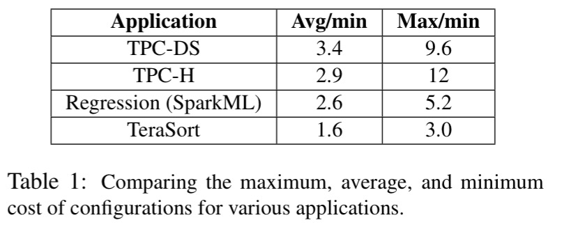
The first results column in the table above shows the mean cost of running the job as it compares to the minimal cost configuration (e.g., for TPC-DS there exists a configuration that is 3.4x cheaper than the average). The second results column shows the ratio of the most expensive to least expensive configurations for the same job (e.g., for TPC-H, the most expensive configuration costs 12x more to run the same job as the least expensive).

How do you find the good configurations though? Just on instance types, Amazon EC2 and Microsoft Azure each offer over 40 (GCP offered 18 at the time of writing, plus the ability to customise VM memory and cores). And that’s before we’ve started to experiment with cluster size… An exhaustive search of the space is clearly way too expensive, especially as each data point requires a run of the job.

CherryPick is a system that leverages Bayesian Optimization to build performance models for various applications, and the models are just accurate enough to distinguish the best or close-to-the-best configuration from the rest with only a few test runs. Our experiments on five analytic applications in AWS EC2 show that CherryPick has a 45-90% chance of finding optimal configurations, otherwise near optimal, saving up to 75% of the search cost compared to existing solutions.

Optimisation challenges

Finding the best configuration is challenging for a number of reasons (even if we can agree on a definition of best : fastest? cheapest? cheapest within some run time bound? fastest within some budget?):

• Runtime may respond in a non-linear way to the amount of resources provided (e.g., Amdahl’s law)
• Cost does not monotonically increase or decrease when adding more resources, since adding resources may accelerate the computation as well as increase the price per unit of running time
• Performance under cloud configurations is not deterministic – results with the same configuration can vary across runs due to stragglers, noisy neighbours and other quirks.
• Different applications respond in very different ways, so general models aren’t very useful

CherryPick’s definition of best by the way, is the lowest cost configuration with a run time less than some specified upper bound. If is a cloud configuration vector (num instances, instance family type, CPU, RAM, and so on), is the running time function for a given application and input workload when using that configuration, and is the price per unit time for the configuration, then we can model the problem as minimising the cost subject to the maximum running time constraint.

Introducing Bayesian Optimisation

In our problem, the ultimate objective is to find the best configuration. We also have a very restricted amount of information, due to the limited runs of cloud configuration we can afford. Therefore, the model does not have enough information to be an accurate performance predictor… [but] we just need a model that is accurate enough for us to separate the best configuration from the rest.

An approach called Bayesian Optimisation (BO) allows CherryPick to adapt its search scheme based on the current confidence interval of the performance model, and to estimate the best next configuration to try to best distinguish performance across configurations. In Bayesian optimisation the true objective function ()is unknown, but we can observe it (sample it) at points through experiments. Modelling as a stochastic Guassian process means we can compute confidence intervals for according to those samples.

A confidence interval is an area that the curve of the objective function is most likely (e.g., with 95% probability) passing through.

An acquisition function also gets updated alongside the confidence interval with each new data point. The acquisition function is used to determine which point to sample next. We’ll look at CherryPick’s choice of acquisition function shortly…

Here’s a worked example. Imagine we have taken two samples at and and computed confidence intervals shown by the blue shaded area below (the dashed line represents the true, unknown, objective function):

We then take a new sample at the point where the acquisition function was maximal, and use this to update the confidence interval and acquisition function:

We can repeat this process until we are satisfied, e.g.:

Our choice of starting points should give BO an estimate about the shape of the cost model. For that, we sample a few points (e.g., three) from the sample space using a quasi-random sequence. Quasi-random numbers cover the sample space more uniformly and help the prior function avoid making wrong assumptions about the sample space.

CherryPick stops when the expected improvement is less than a threshold (e.g. 10%), and at least N (e.g., N = 6) configurations have been observed.

To help further reduce the search space, most of the features in are normalized and discretized. For example, for disk speed only ‘fast’ and ‘slow’ are defined to distinguish SSDs and magnetic disks.

Modelling the prior function

The Gaussian process it is described with a mean function and a covariance function. If two cloud configurations are similar to each other, we expect high covariance, and if they are dissimilar they should have low covariance. The authors chose the  Matérn 5/2 function for this “because it does not require strong smoothness, and is preferred to model practical functions.”

See section 3.6 for details of how CherryPick deals with noise in the underlying cloud platform. In brief, we don’t want to do multiple tests of each configuration due to the expense, so CherryPick models noise via a multiplicative noise factor &eps;, assumed to be less than one. Then it becomes possible to use BO to optimise instead of and everything works out.

Modelling the acquisition function

CherryPick uses Expected Improvement (EI) for its acquisition function – picking the point which can maximise the expected improvement over the current best. See eqn (3) in section 3.5 of the paper for the detail, which is based on “an easy-to-compute closed form for the EI acquisition function” from Jones at al., “Efficient global optimization of expensive black box functions.”

CherryPick end-to-end

The entire CherryPick system is 5000 lines of Python code (not counting the Spearmint BO library it uses).

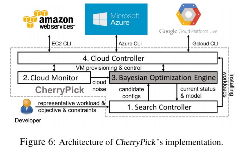
• The search controller orchestrates the overall process, allowing the user to specify workload, the objective, and constraints and passing these to the Bayesian Optimisation Engine.
• The cloud monitor runs benchmark workloads on different clouds to measure the upper bound for cloud noise. The result determines the noise multiplication factor, ε passed to the optimisation engine.
• The Bayesian optimisation engine is built on top of the Spearmint BO library.
• The cloud controller abstracts over differing cloud provider interfaces

Evaluation

CherryPick is evaluated with a variety of Spark and Hadoop benchmark applications: TPC-DS, a decision support workload on Spark SQL; TPC-H, an ad-hoc decision support workload on Hadoop; TeraSort, a big data analytics benchmark on Hadoop; SparkReg machine learning workloads on Spark; and SparkKm, a SparkML benchmark. Tests are done on EC2 using four instance families:

1. M4 (general purpose)
2. C4 (compute optimised)
3. R3 (memory optimised)
4. I2 (disk optimised)

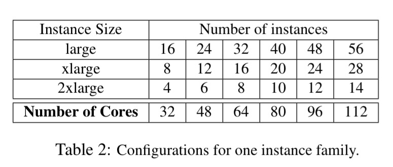
Within each family, large, xlarge and 2xlarge instance sizes are used. Overall 66 different configurations are tested for each family:

The evaluation considers how good the best found configuration is, and how expensive it was to find it. Exhaustive search is used as a comparison, so that we can assess the configuration recommended by CherryPick against the best possible choice. Here are the key findings:

• CherryPick can find the optimal configuration 45-90% of the time, and if it doesn’t find the absolute best, it will find a near-optimal configuration, with low search cost and time. For example, with the TeraSort workload running exhaustive search costs $630, while CherryPick costs $195.

• CherryPick finds better solutions than a random search (sanity check!): here you can see the running times of solutions found by CherryPick against random search given the same, 2x, and 4x the search budget.

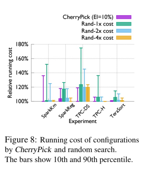
• Users can tune CherryPick to trade-off between search cost and quality of the discovered configuration.

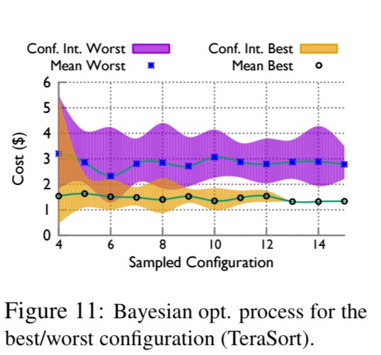
You can see in the following chart how the mean and confidence intervals for the best and worst configurations discovered so far are refined during a sample Bayesian optimisation of the TeraSort workload:

CherryPick adapts its search towards features that are more important to the application. The following example search paths show CherryPick homing in on instances with larger RAM (R3 instances) for SparkReg, while favouring instances with better CPUs (C4 instances) for TPC-DS.

And this illustration shows how CherryPick learns the relation between cloud resources and running time:

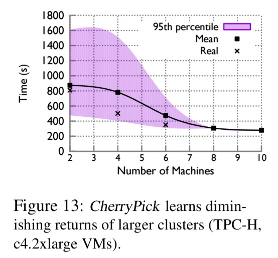
The real curve follows Amdahl’s law: (1) adding more VMs reduces the running time; (2) at some point, adding more machines has diminishing returns due to the sequential portion of the application… CherryPick has smaller confidence intervals for the more promising region where the best configurations (those with more VMs) are located. It does not bother to improve the estimation for configurations with fewer VMs.