Explaining outputs in modern data analytics Chothia et al. ETH Zurich Technical Report, 2016

Yesterday we touched on some of the difficulties of explanation in the context of machine learning, and last week we looked at some of the extensions to ExSPAN to track network provenance. Lest you be under any remaining misapprehension that explanation (aka provenance) is a straightforward problem, today’s paper looks at the question of provenance in dataflow systems. Sections 2.1 (‘Concepts of data provenance’) and 5 (‘Related work’) also provide some excellent background and pointers to other work in the space. I’ve linked to the formal technical report above, but Frank McSherry also has an excellent blog post describing the work which I highly recommend. He writes with a wit and verve I cannot hope to match!

… we provide a general method for identifying explanations that are sufficient to reproduce the target output in arbitrary computations – a problem for which no viable solution existed until now.

Concepts and background

The basic idea of provenance is to explain how the outputs of a computation relate to its inputs. Initial work started in database systems under the term data lineage, later broadened to data provenance. A provenance graph shows the flow of individual tuples en route from inputs to outputs. For example:

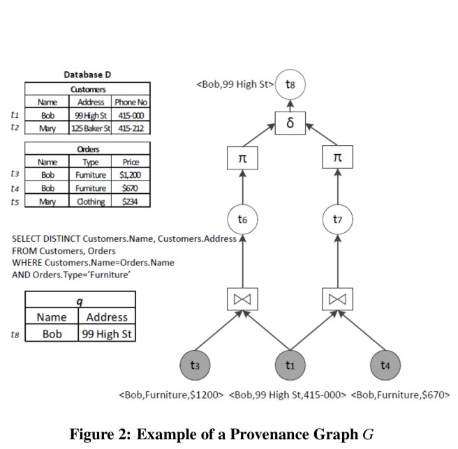
• The lineage of t₈ is the highlighted tuples { t₁, t₃, t₄ }.
• The why provenance of t₈ is the multi-set {{ t₁,t₃}, {t₁,t₄}}. Each of the two subsets being a proof or witness for the presence of t₈ in the output.
• The how provenance of t₈ is “t₁ and (t₃ or t₄)”, which would be easy to understand written as but is expressed as a semi-ring (where ‘.’ is and and ‘+’ is or).
• Transformation provenance describes all the possible ways of having t₈ in the output – it adds the actual query operators involved in the process on top of what we get in the why provenance. The graph above is an example of transformation provenance.
• Where provenance is defined at the attribute level, so for example the where provenance of t₈.Address is t₁.Address.

In establishing provenance we’d ideally like concise explanations. Consider an explanation for a connected components computation, and we want to explain why a given node B receives the same label as a node A. If we did a straightforward backward tracing, in which each operator in a dataflow graph maintains a reverse mapping from its output records to its input records, we’d end up implicating the whole connected component in the explanation. A better explanation would be: “because there’s an edge from A to B.”

So too much information can be a problem. But we also have to be careful not to provide too little information. A particular trap here is when we have non-monotonic data transformations. That is, we can add additional inputs which suppress some of the former outputs. Consider a map-reduce dataflow for a unique word count. If we add a new document as input, some words which were previously unique may no longer be.

In ‘Explaining outputs in modern data analytics’, Chotia et al. give us (a) a backward tracing approach that identifies concise explanations for an output record of an arbitrary iterative computation, based on the first occurrence of the record in the computation, and (b) explanations sufficient to reproduce the output in an arbitrary, even iterative, dataflow with any combination of monotonic and non-monotonic operators.

Backward tracing in differential dataflow – the core idea

The work is set in the context of differential dataflow , a data-parallel programming and execution model layered on top of Naiad’s timely dataflow. One important piece of background is that differential dataflow provides for iterative incremental execution of operators.

The framework we present relies on the ability of differential dataflow to efficiently execute and update iterative data-parallel computations. Explanations are produced by iteratively updating a fixed-point implementation of backward tracing. Differential dataflow not only efficiently computes these explanations, but it also updates them automatically as the source computation changes.

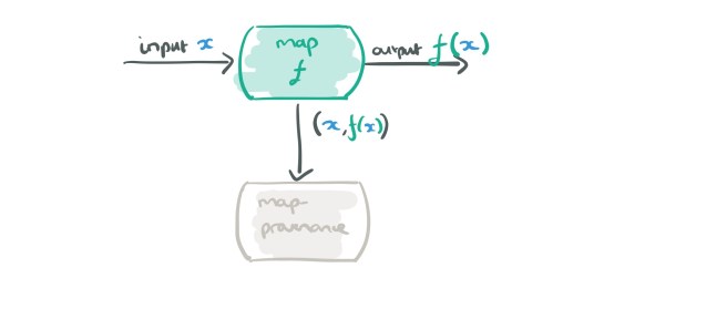
Consider for a moment just the map and reduce operators, and records flowing in a dataflow graph that are (key, payload) pairs (like a key-value pair, but the payload can also contain metadata). Let’s look at a map node in a dataflow graph, which applies some function f to its input data d, giving output f(d).

To capture provenance, we want to record the (input, output) pairs from the map operator. We could just send them off to some external provenance recording system, but there’s a better way. We could send them to a provenance collecting dataflow operator instead…

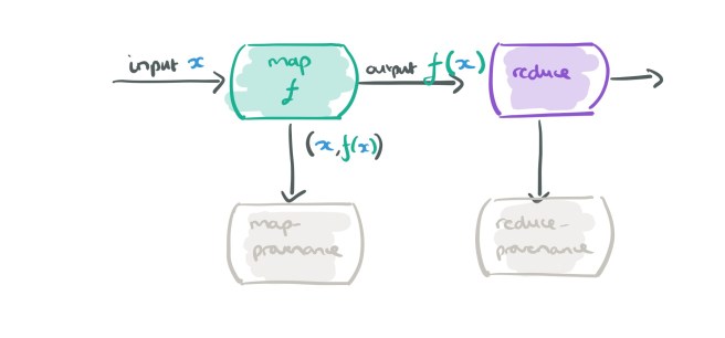
Let’s add a reduce stage into the mix, which also sends its (input, output) information to its own provenance collecting dataflow operator:

And here comes the clever bit… when we are recording provenance for the map operator, we don’t actually need to record all input, output pairs, we just want those that are needed to explain the ultimate output of the dataflow. Which pairs are they? Just the ones needed to explain the outputs of its downstream operators (i.e., the reduce in this case). So we can feed those into our provenance mapper and do a streaming join.

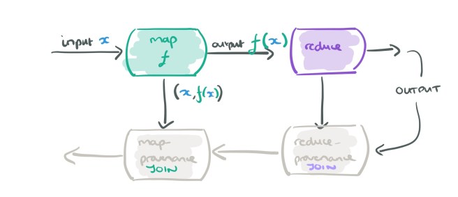
The end result is a shadow dataflow graph that maps the original computation but where information flows in the opposite direction.

Expressing the explanation logic as a join that matches queried outputs against explanatory inputs has two major advantages. First, we do not rely on specialized data structures for maintaining provenance; hence; our approach can be easily incorporated into any system. Second, the explanation join can be implemented as a data-parallel operator itself to achieve robust and scalable provenance querying.

The shadow provenance operators do maintain a second copy of the input in the general case (which can be expensive), but for several common data transformations this overhead can be reduced (see the full paper for invertible map, top-k, and join examples).

… the most important change we make in our explanation logic is that the inputs of an operator can be restricted to those with logical timestamp less-or-equal to that of the required output. This allows us to … substantially reduce the volume of records in the reported provenance.

Iterative backward tracing

Thus far we have succinct and efficient explanations, but what about the tricky case on non-monotonic outputs? The input records identified by backwards tracing as described so far may not be sufficient to explain these. We do know that to affect the output there must be some intermediate records interfering in downstream computations. Therein lies the clue:

Although it appears difficult to identify the records that deviate from the reference computation early, we can discover them through their main defective property: to affect the output they must intersect the backwards trace. If we maintain a second instance of the computation, re-executed only on the inputs identified by the backwards trace, then any new records it produces that intersect the backwards trace can themselves be traced backwards, and ultimately corrected through the introduction of more input records.

Space precludes me from detailing the results of the evaluation, but §4 of the paper contains some nice examples of datalog provenance, connected components, and stable matching provenance (exhibiting the non-monotonic property) together with the overheads introduced by capturing provenance as the computations proceed.

The experiments indicate that our framework is suitable for a variety of data analysis tasks, on realistic data sizes, and with very low overhead in performance, even in the case of incremental updates.

Related work

Section 5 of the paper has some very nice pointers to related work, of especial interest to me is the work on tracking provenance in NoSQL systems: RAMP, Newt, and Titian. You’ll also find a discussion of ExSPAN that we looked at last week.

Here’s a handy summary table of NoSQL systems with provenance support and how they stack up:

So is provenance solved now???

We believe that our approach is here to stay and there are several directions for future work. Besides the further optimization opportunities, we are especially interested in understanding the structure of explanations for general data-parallel computations; while our intuition serves us well for tasks like graph connectivity, our understanding of explanations for problems like those in ‘Scaling datalog for machine learning on big data‘ has huge potential for improvement.

And what about the explanations required by the GDPR? For this use case, do we have to retrofit provenance mechanisms such as the above to all of our systems? If we have to explain a particular output (decision impacting a person) at a particular point in time, perhaps yes. But returning to the ‘unique word count’ example, a human-understandable general explanation is “we return all words that are unique across all input documents.” And maybe that is good enough? My understanding of the current status quo is that we just don’t know!