Matching networks for one shot learning Vinyals et al. (Google DeepMind), NIPS 2016
Yesterday we saw a neural network that can learn basic Newtonian physics. On reflection that’s not totally surprising since we know that deep networks are very good at learning functions of the kind that describe our natural world. Alongside an intuitive understanding of physics, the authors of “Building machines that learn and think like people” also called out one-shot learning as a capability which humans have and which machine learning systems struggle with. Today’s paper choice sees the Google DeepMind team take on that challenge:
Learning from a few examples remains a key challenge in machine learning. Despite recent advances in important domains such as vision and language, the standard supervised deep learning paradigm does not offer a satisfactory solution for learning new concepts from little data.
Suppose I say to you “a Rebra is a Zebra but with red and white stripes,” and then show you a sample image. You’d then be able to tell me which other pictures had Rebras in them. The one-shot learning challenge is similar: the system is shown a single labelled example and from this it should be able to learn to detect other examples of the same class.
Deep learning isn’t very good at this – it needs lots of examples to drive lots of iterations of stochastic gradient descent and gradually refine the weights in the model. In contrast, something like k-nearest neighbours (KNN) doesn’t require any training at all. Suppose we see only 1 example of a class as in one-shot learning. If we used 1-NN and thus predicted the class of a previously unseen input as its nearest neighbour we’d have a basic system. Unfortunately it probably wouldn’t work very well in the real world, and we still have the problems of learning a good feature representation and choosing an appropriate distance function.
The Matching Nets architecture described in this paper blends these two extremes, using neural networks augmented with memory (as we saw for example in Memory Networks and the Neural Turing Machine). In these models there is some external memory and an attention mechanism which is used to access the memory. It’s a network that learns how to learn a classifier from only a very small number of examples…
A matching network is shown a support set S of k labelled examples with input x and label y : . Given a new example
we want to know the probability that it is an instance of a given class:
. The probability function P is parameterised by a neural network. Given such a function, predicting the output class becomes as simple as
. In plain English, predict the output class with the highest probability. So far, this reads pretty much like a mathematical redefinition of the problem. The secret lies in how P is formulated. Given an input
, a matching network model computes the estimated output label
as follows:
(1)
Here is an attention mechanism and its role is to specify how similar
is to
. Think of it as a kind of fuzzy associative memory from
. Note that
is a linear combination of the labels in the support set (we sum over all examples, i = 1..k). What does it mean to take a linear combination of labels? I.e., what is 0.7 x cat + 0.2 x dog ?? It took me a good while to figure that out – my interpretation is that the input
must be one-hot vectors, in which case we end up with a probability distribution over labels again (0.7 x [0,1] + 0.2 x [1.0]). Thanks to Oriol Vinyals (the first author) for subsequently confirming on twitter that this is indeed the case! Obvious with hindsight…
For the attention mechanism itself, the authors use the cosine distance between and
, passed through a softmax (to normalise distances between 0 and 1). We also need to map (lift) from the input space to the feature space in which we will do the distance comparisons. Functions f and g can do that for us.
Plugging into the softmax formula:
we get

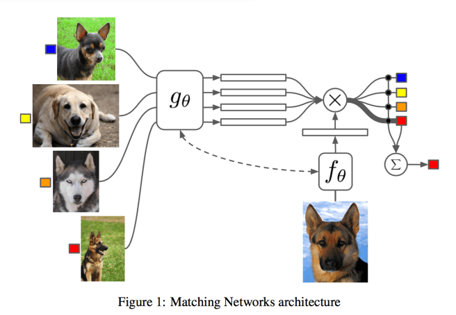
At this point a picture is probably very helpful:

You’re probably wondering why we use different embedding functions for and
since they’re both of the same type (e.g., both images). The function g (for embedding the examples from S) takes the full set S in addition to the element x , i.e., it becomes
. This is done to allow g to modify the way it embeds
based on what else is in the set – for example, there might be some other
very close to it. The encoding function g is modelled as a bidirectional LSTM. In a similar manner f is also passed the whole set S and can use that knowledge to change how it encodes
.
You get good at what you practice
If you want to become good at learning a classifier given only a very small number of examples, then it makes sense to train that way!
To train a matching net, first sample a small number of labels (e.g., the set {cats, dogs}), and then sample a support set S with a small number of examples per label (e.g. 1-5), and a batch B to be used to training.
The Matching Net is then trained to minimise the error predicting the labels in the batch B conditioned on the support set S. This is a form of meta-learning since the training procedure explicitly learns to learn from a given support set to minimise a loss over a batch.
Experiments
Matching Networks were tested on a number of N-way (N labels/classes), k-shot (k examples per class) learning tasks. Data sets were drawn from the Omniglot and ImageNet image data sets, and the Penn Treebank language modelling data set.
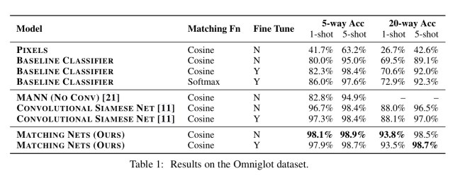
Omniglot contains 1623 characters from 50 different alphabets, each hand-drawn by 20 different people. A CNN was used as the embedding function. In both 1-shot and 5-shot, 5-way and 20-way tests, Matching Networks outperform a baseline of the state-of-the-art MANN classifier, as well as a Convolutional Siamese Net (neither of these were designed for one-shot learning of course).

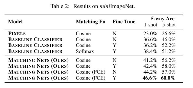
A variety of experiments were performed with the ImageNet dataset. The miniImageNet test used 60,000 images with 100 classes, each having 600 examples. 80 classes were used for training, and testing was done on the other 20. Here are a couple of examples of Matching Networks classifying in a 5-way test (vs the Inception baseline):

Here are the detailed results:

Note the row labelled ‘FCE’, which stands for ‘Full Contextual Embedding’ (i.e., passing S into g and f) – which turns out to be worth about 2 percentage points for one-shot learning on this task.
The language task is to take a query sentence with a missing word, and predict the missing word (class). The support set contains sentences with a missing word and corresponding label for the missing word. An LSTM oracle which sees all the data (i.e., is not one-shot) defined an upper bound for this task of 72.8% accuracy. Matching Networks achieved 32.4%, 36.1%, and 38.2% accuracy with k = 1, 2, 3.
In this paper we introduced Matching Networks, a new neural architecture that, by way of its corresponding training regime, is capable of state-of-the-art performance on a variety of one-shot classification tasks. There are a few key insights in this work. Firstly, one-shot learning is much easier if you train the network to do one-shot learning. Secondly, non-parametric structures in a neural network make it easier for networks to remember and adapt to new training sets in the same tasks.
(Non-parametric here is referring to the use of the memory, as opposed to having to try and encode everything that has been seen solely in trained weights).

I read the paper and was extremely puzzled about the weighted sum of labels. That didn’t make sense to me. But yeah, something like 0.2[1,0,0] + 0.5[0,1,0] + 0.3[0,0,1] = [0.2,0.5,0.3] makes total sense. I wish this had been clearer in the paper. Also, the softmax here is over cosine distance between \hat{x} and all x_i in the support set. I’m guessing this becomes extremely expensive when the support set gets large?
I think the whole point of the paper is to train incrementally with very less data. That kind of hints at not having support sets too large (equivalent to the situation a human has).
Sorry, another question, so for miniImageNet, they tested on 20 labels. Based on what I understood of the paper, this means the model learns to classify images on 20 labels that it has actually *never* seen in training? And it’s able to do that because it has learned how to embed inputs and learned how to match one sample with another sample? Amazing.
I am also confused by “80 classes were used for training, and testing was done on the other 20”. The paper does not make it clear the problem they want to solve. They also did not compare their method with conventional one-shot learning methods. If you read the NIPS reviews, several reviewers criticize the paper is very unclear. It is amazing such a paper can be published on NIPS. Disappoint.
Can you give the link and reviewer number? I’ll have a look
The review cna be found here: https://media.nips.cc/nipsbooks/nipspapers/paper_files/nips29/reviews/1804.html
This paper gives an impressively successful combination of techniques, but fails a bit to pay tribute to its predecessors. For the reference, equation (1) is refered to as Shepard’s method in “Lifelong Learning Algorithms” by Thrun (1998), the idea to read one-shot training samples as a sequence is I believe introduced by “Learning to Learn Using Gradient Descent” by Hochreiter (2001).
Hi,
Thanks for your article. I helps me a lot to understand the paper.
I have a question though: A support set S have K examples per label, and increasing K helps improve the model performance. This confuses me because I thought a support set should have only 1 example per label. Why? If it has more than 1 examples per label class, the attention might not make much sense because it will give more attention to an example in a label class and give less attention to the others in a label class. I mean, I thought the goal of attention mechanism is to give more attention to a specific label class and less attention to other label classes instead.
I hope I made my question clear.
Thanks a lot!