Serverless in the wild: characterizing and optimising the serverless workload at a large cloud provider, Shahrad et al., arXiv 2020
This is a fresh-from-the-arXivs paper that Jonathan Mace (@mpi_jcmace) drew my attention to on Twitter last week, thank you Jonathan!
It’s a classic trade-off: the quality of service offered (better service presumably driving more volume at the same cost point), vs the cost to provide that service. It’s a trade-off at least, so long as a classic assumption holds, that a higher quality product costs more to produce/provide. This assumption seems to be deeply ingrained in many of us – explaining for example why higher cost goods are often implicitly associated with higher quality. Every once in a while though a point in the design space can be discovered where we don’t have to trade-off quality and cost, where we can have both a higher quality product and a lower unit cost.
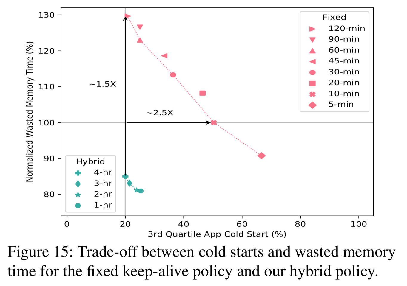
Today’s paper analyses serverless workloads on Azure (the characterisation of those workloads is interesting in its own right), where users want fast function start times (avoiding cold starts), and the cloud provider wants to minimise resources consumed (costs). With fine-grained, usage based billing, resources used to keep function execution environments warm eat directly into margins. The authors demonstrate a policy combining keep-alive times for function runtimes with pre-warming, that dominates the currently popular strategy of simply keeping a function execution environment around for a period of time after it has been used, in the hope that it will be re-used. Using this policy, users see much fewer cold starts, while the cloud provider uses fewer resources. It’s the difference between the red (state-of-the-practice) and green (this paper) policies in the chart below. Win-win!
We propose a practical resource management policy that significantly reduces the number of function cold starts, while spending fewer resources than state-of-the-practice policies.
Before we get to how the policy works, first lets take a look at what the paper tells us about real production serverless workloads on Azure (all function invocations across all of Azure, July 15th-28th, 2019). Those insights inform the policy design.
###Serverless in the real world, a service provider’s perspective
The dataset includes invocation counts, execution times, memory usage, and metadata (e.g., trigger type) for every function invoked across Azure for the days in question. In Azure functions are logically grouped in applications, and its the application that is the unit of scheduling and resource allocation.
Over half of all apps have only one function, 95% have at most 10 functions, and 0.04% have more than 100 functions. Looking at invocations overall, the number of functions within an applications turns out not to be a useful predictor of invocation frequency. Applications with more functions show only a very slight tendency for those functions to be invoked more often. The most popular way to trigger a function execution is an HTTP request. Only 2.2% of functions have an event-based trigger, but these represent 27.4% of all invocations. Meanwhile many functions have a timer-based trigger, but they only account for 2% of all invocations. I.e., events happen much more frequently than timer expiry!
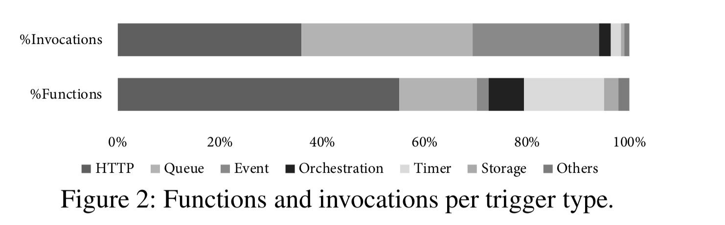
Timer-based triggers are great for predicting when a function will be invoked, but 86% of applications either have no timer, or have a combination of timer and other triggers.
The number of invocations per day can vary by over 8 orders of magnitude across functions and applications, implying very different levels of resource requirements.
… the vast majority of applications and functions are invoked, on average, very infrequently… 45% of applications are invoked once per hour or less on average, and 81% of the applications are invoked once per minute or less on average. This suggests that the cost of keeping these applications warm, relative to their total execution (billable) time, can be prohibitively high.
An analysis of the inter-arrival times (IATs) of those function executions shows that real IAT distributions are more complex than simple periodic or memoryless distributions. For many applications, predicting IATs is not trivial.
When functions do execute, the amount of time they execute for is comparatively short (50% of functions execute for 1s or less).
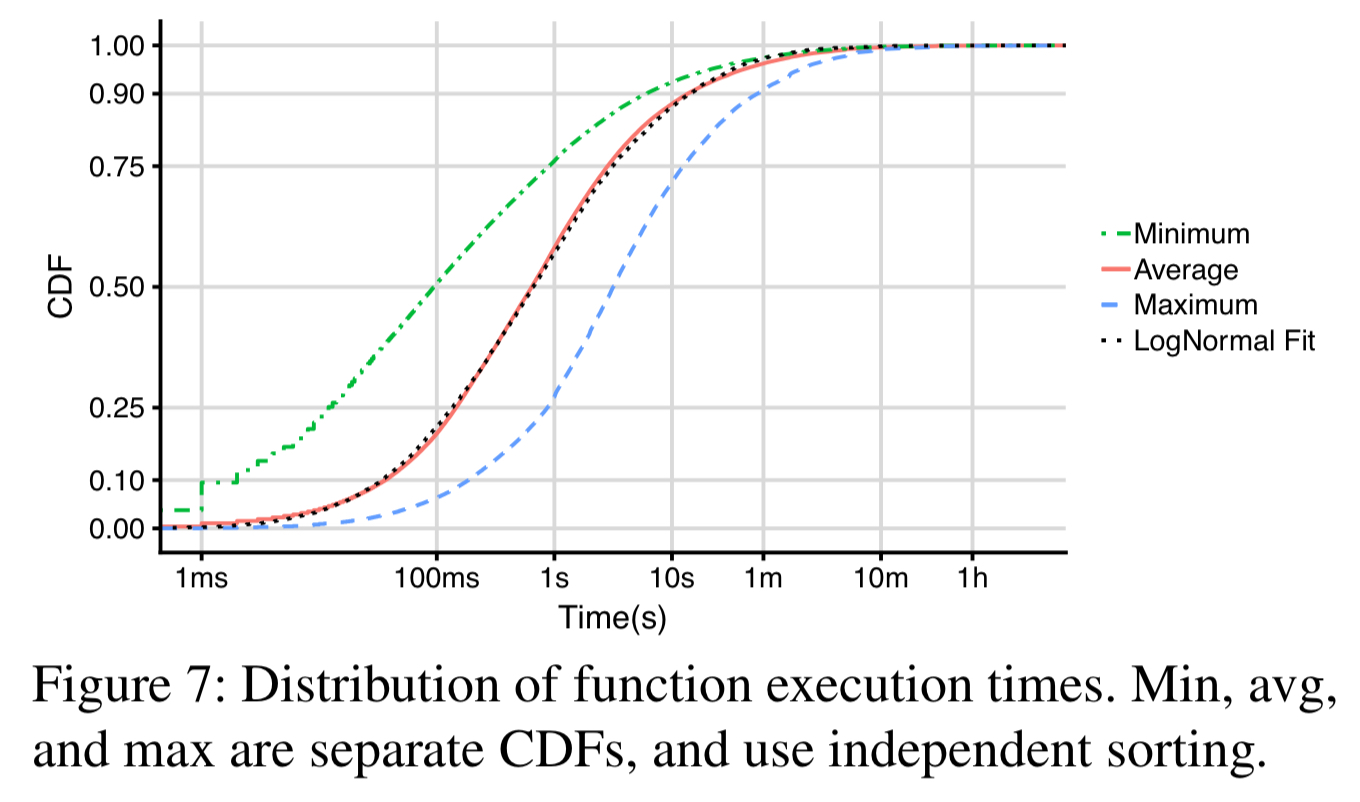
The main implication is that the function execution times are at the same order of magnitude as the cold start times reported for major providers. This makes avoiding and/or optimizing cold starts extremely important for the overall performance of a FaaS offering.
Moreover, for most applications the average execution time is at least two orders of magnitude smaller than the average IAT.
There is also wide variation in memory consumption, but no strong correlation between invocation frequency and memory allocation, or between memory allocation and execution time.
In short, most functions are invoked infrequently with short lifetimes, and it’s expensive to keep these resident. But the task of predicting when a function will next be invoked is non-trivial.
When and how long to keep a function execution environment alive
From a service provider perspective, there are two important questions that govern application performance and resource consumption:
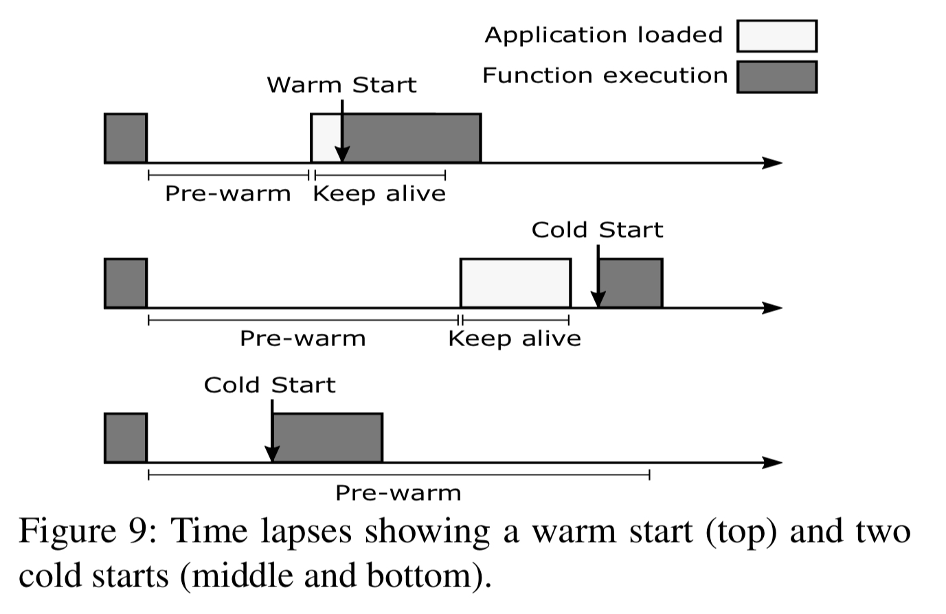
- When (if at all) should an application execution enviroment be pre-warmed in anticipation of a forthcoming invocation, and
- After an application execution environment has been loaded into memory, how long should it be kept alive for (keep-alive). (Not this definition starts from the moment of pre-warming, if an application is pre-warmed)
The answers to these questions need to be different for each application as we have seen. In the absence of any strong correlations we can piggy-back off of, that means we need to learn the behaviour of each function – but we need to do so with low tracking and execution overheads.
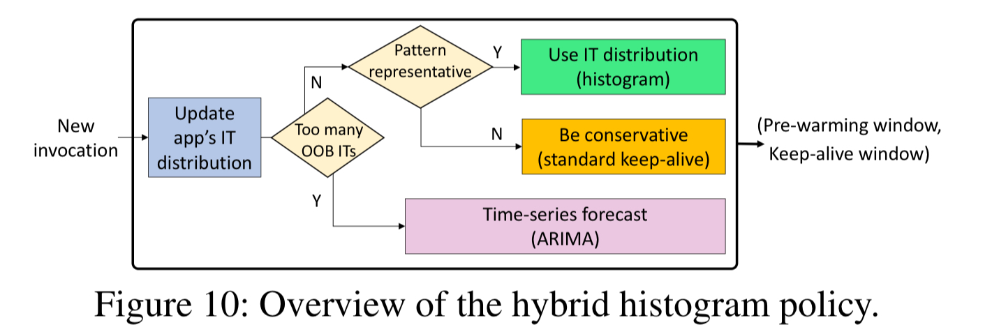
The solution is a hybrid histogram policy that adjusts to the invocation frequencies and patterns of each application. It has three main components:
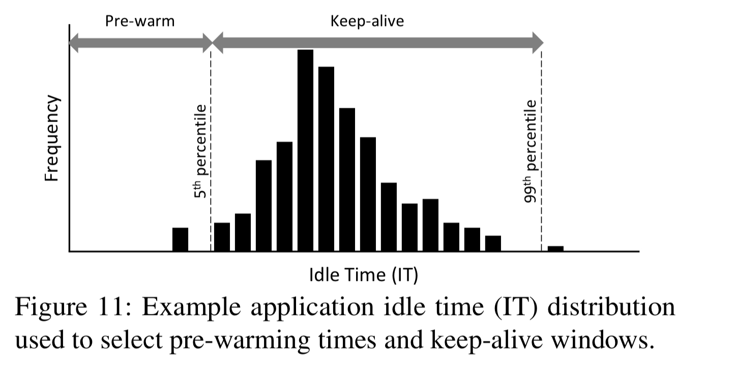
- A range-limited histogram capturing idle time (IT) distribution for each application. Each 1-minute wide bin captures the number of ITs of the corresponding length that have occured, for ITs of up to 4 hours. The head of this distribution (taken at the 5th percentile) is used to set the pre-warming window, and the tail (taken at the 99th percentile) is used to set the keep-alive window.
- A standard keep-alive policy used when not enough ITs have been observed yet, or the IT distribution is undergoing change. The histogram is most effective when the coefficient of variation is higher than some threshold. Below this the standard keep-alive is used, which has no pre-warming and a four-hour keep-alive time. "This conservative choice of keep-alive window seeks to minimize the number of cold starts while the histogram is learning a new architecture."
- When an application experiences many out-of-bound (more than 4 hour) idle times the histogram approach is never going to work well. For these applications a more expensive ARIMA model is used to predict idle time. This model is computed off the critical path, and only needed for a minority of invocations so computation needs are manageable.
It all comes together like this:
The hybrid policy in action
The hybrid policy is evaluated both with a simulation based on the full Azure trace, and an Open Whisk based implementation replaying a section of it. We saw one of the headline results at the top of this post in Fig 15: the hybrid policy significantly reduces the number of cold starts while also lowering memory waste.
The 10-minute fixed keep-alive policy [current cloud provider approach] involves ~2.5x more cold starts at the 75th percentile while using the same amount of memory as our histogram with a range of 4 hours… Overall, the hybrid policies form a parallel, more optimal Pareto frontier (green curve) than the fixed policies (red curve).
If you’re interested in diving deeper, the evaluation also shows the contribution made by the histogram range-limiting, by the checking of histogram representativeness to fall back to the standard keep-alive policy, and by the use of ARIMA models of out-of-bound idle time applications.
We achieve these positive results despite having deliberately designed our policy for simplicity and practicality: (1) histogram bins have a resolution of 1-minute, (2) histograms have a maximum range, (3) they do not require any complicated model updates, and (4) when the histogram does not work well we revert to simple and effective alternatives.
Coming soon to a cloud provider near you no doubt!

> ###Serverless in the real world, a service provider’s perspective
A space maybe missing here.