Large scale GAN training for high fidelity natural image synthesis Brock et al., ICLR’19
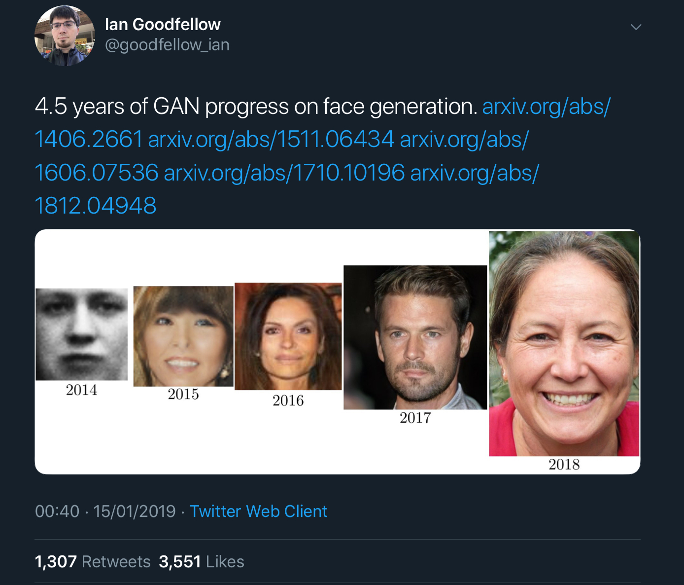
Ian Goodfellow’s tweets showing x years of progress on GAN image generation really bring home how fast things are improving. For example, here’s 4.5 years worth of progress on face generation:
And here we have just two years of progress on class-conditional image generation:
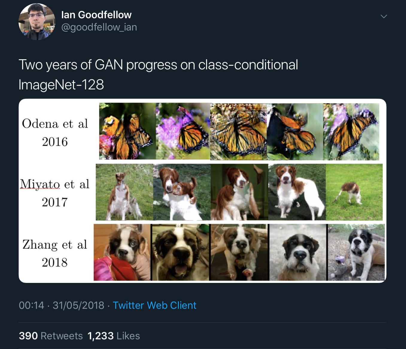
In the case of the faces, that’s a GAN trained just to generate images of faces. The class-conditional GANs are a single network trained to generate images of lots of different object classes. In addition to feeding it some noise (random input), you also feed the generator network the class of image you’d like it to generate (condition it).
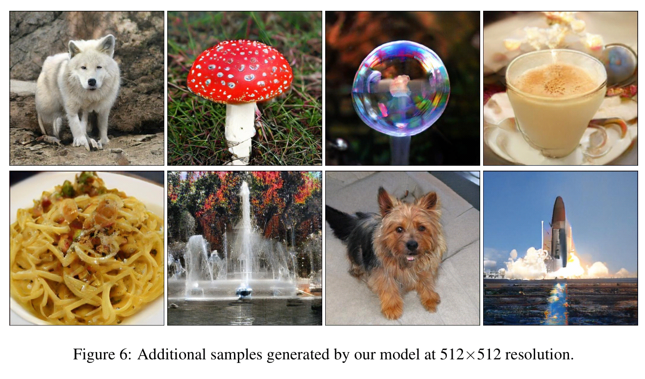
I was drawn to this paper to try and find out what’s behind the stunning rate of progress. The large-scale GANs (can I say LS-GAN?) trained here set a new state-of-the-art in class-conditional image synthesis. Here are some images generated at 512×512 resolution.
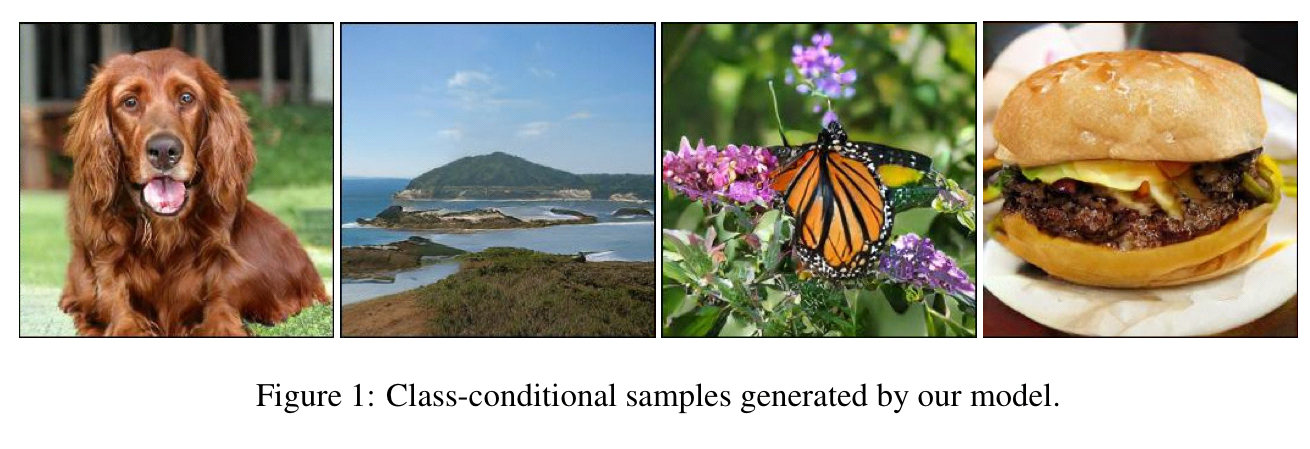
The class-conditional problem is of course much harder than the single image class problem, so we should expect the images to be not quite so stunning as the pictures of faces. In fact, using a measure called the Inception Score, the best result prior to this paper achieved a score of 52.5, whereas real data scores 233. LS-GAN closes the gap considerably with a score of 166.3. You can see in these images that for some classes well represented in the training set (e.g. dogs), the pictures look very good. For others it’s still easy to tell the images are generated (e.g., the butterfly isn’t quite right, and the burger seems to have a piece of lettuce that morphs into melted cheese!).
So what’s the secret to LS-GANs success? Partly of course it’s just a result of scaling up the models – but interestingly by going wide rather than deep. However, GANs were already notoriously difficult to train (‘unstable’), and scaling things up magnifies the training issues too. So the other part of the innovation here is figuring out how to maintain stability at scale. It’s less one big silver bullet, and more a clever aggregation of techniques from the deep learning parts bin. All in all, it has the feel to me of reaching the upper slopes of an ‘s’-curve such that we might need something new to get us onto the next curve. But hey, with the amazing rates of progress we’ve been seeing I could well be wrong about that.
We demonstrate that GAN’s benefit dramatically from scaling, and train models with two to four time as many parameters and eight times the batch size compared to prior art. We introduce two simple, general architectural changes that improve scalability, and modify a regularization scheme to improve conditioning, demonstrably boosting performance.
How good are the generated images?
If we’re going to talk about the performance of a GAN, we need some measure of the quality of the images it creates. There are two dimensions of interest here: the quality of the samples, and the diversity of the generated images. This paper uses both Inception Score (IS) and Fréchet Inception Distance (FID) as quality measures. There’s a good introduction to these two measures in ‘How to measure GAN performance’ by Jonathan Hui. Both scores combine quality and diversity, the Inception Score using the KL-distance between probability distributions, and the FID score using (Gaussian) distribution parameters. For IS, higher scores are better, and for FID lower scores are better.
The starting point
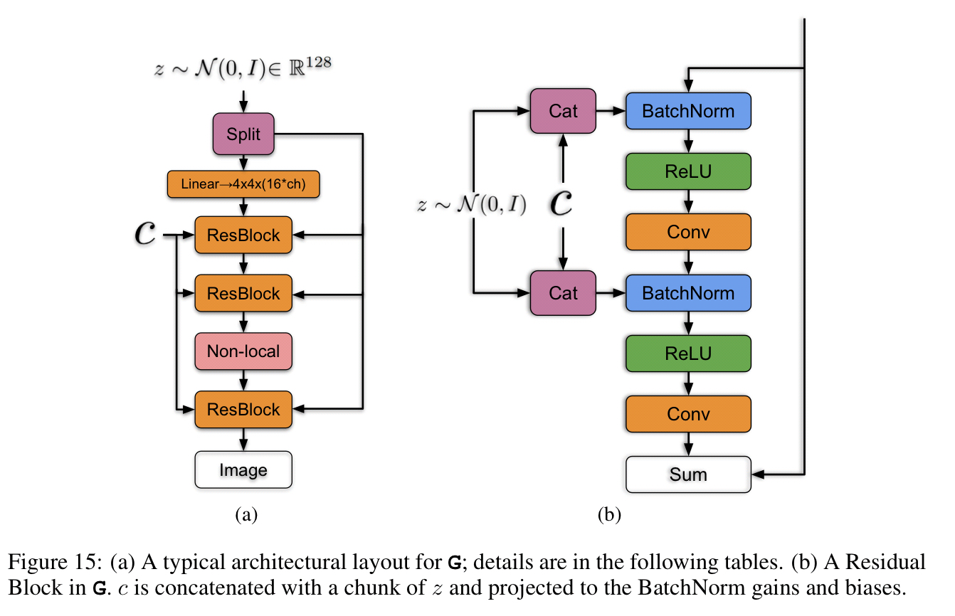
As a baseline the authors start with SA-GAN, which incorporates a self-attention block. The class information is fed into the generator using a class-conditional BatchNorm. (BatchNorm normalises the input features of a layer to have zero mean and unit variance). Spectral normalisation is used for regularisation. In short, this uses as a regularisation term the first singular value of the matrix. Models are trained on 128-512 cores of a Google TPU v3 Pod. Of note is that with this set up progressive growing was found to be unnecessary, even for the largest 512×512 models.
Scaling up
The first enhancement compared to the baseline is to increase the batch size. Increasing batch size by a factor of 8x improves on the state-of-the-art Inception Score by 46%.
We conjecture that this is a result of each batch covering more modes, providing better gradients for both networks.
Using the larger batch sizes the models reach better final performance in fewer iterations, but also tend to become unstable and undergo complete training collapse.
The next move is to increase the width (number of channels) in every layer by 50%. This further improves the Inception Score by another 21%. The gain here is attributed to the increased capacity of the model relative to the complexity of the dataset.
Doubling the depth does not appear to have the same effect on ImageNet models, instead degrading performance.
Further Modifications
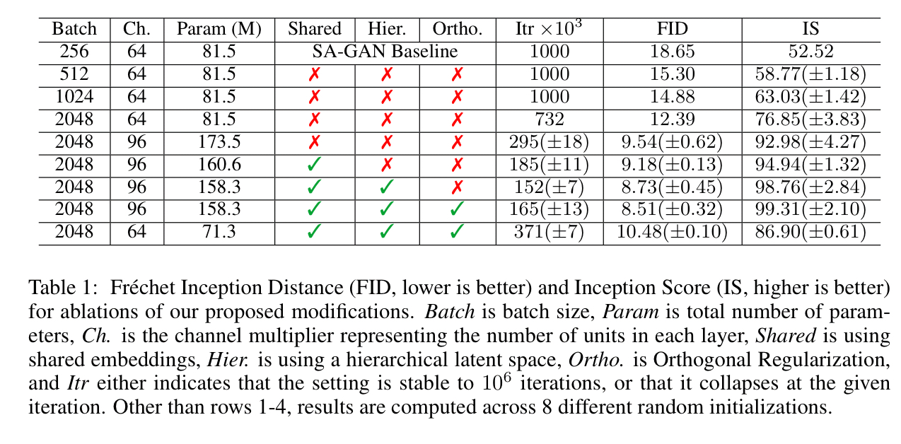
Having a separate layer for each conditional BatchNorm embedding introduces a large number of weights. So LS-GAN uses a single shared embedding which is linearly projected to each layer’s gains and biases. The net result is a 37% improvement in training speed together with reduced memory and computation costs.
Next, the input noise vector is split into chunks, with the different chunks fed into different layers of the network (forming a hierarchical latent space). “The intuition behind this design is to allow the generator to use the latent space to directly influence features at different resolutions and levels of the hierarchy.”
For reasons we’ll see next we’d like the full input space of 

The table below shows how all these modifications stack up in terms of impact on FID and IS scores and training stability:
The ‘truncation trick’
So why did we need that smoothness in the sample space? The authors observe that for the input noise you can draw from any distribution you like. After exploring various options they find that…
Remarkably, our best results come from using a different latent distribution for sampling than was used in training. Taking a model trained with
and sampling
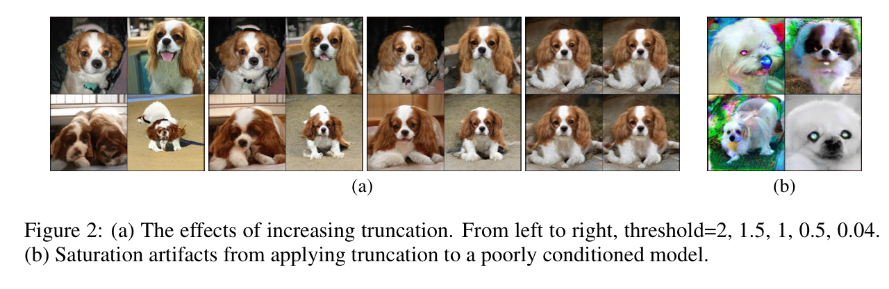
The following figure shows the effects of increasing tighter cutoffs.
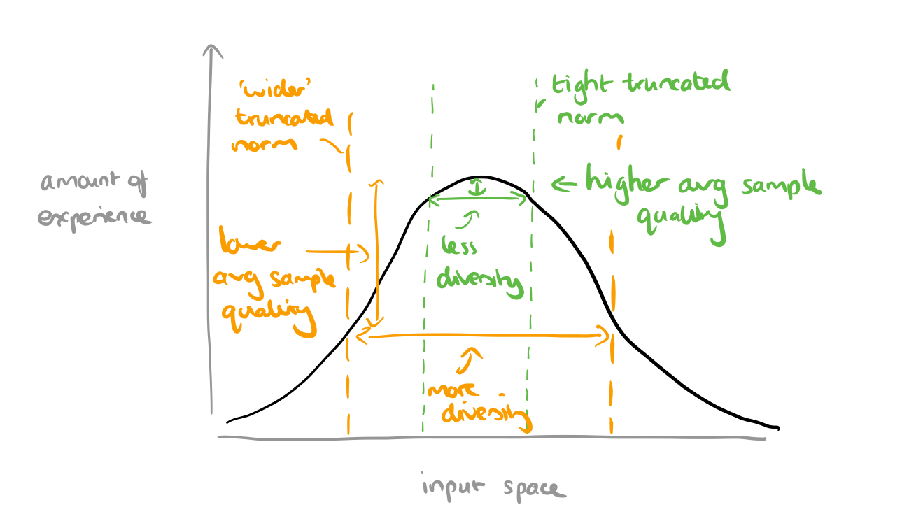
It’s a neat idea, but on reflection it doesn’t seem quite so surprising as the word ‘remarkably’ in the quote above suggests. We’re training with samples drawn from a normal distribution, which means a plot of how much ‘experience’ the model has with different parts of the input space will look like this:
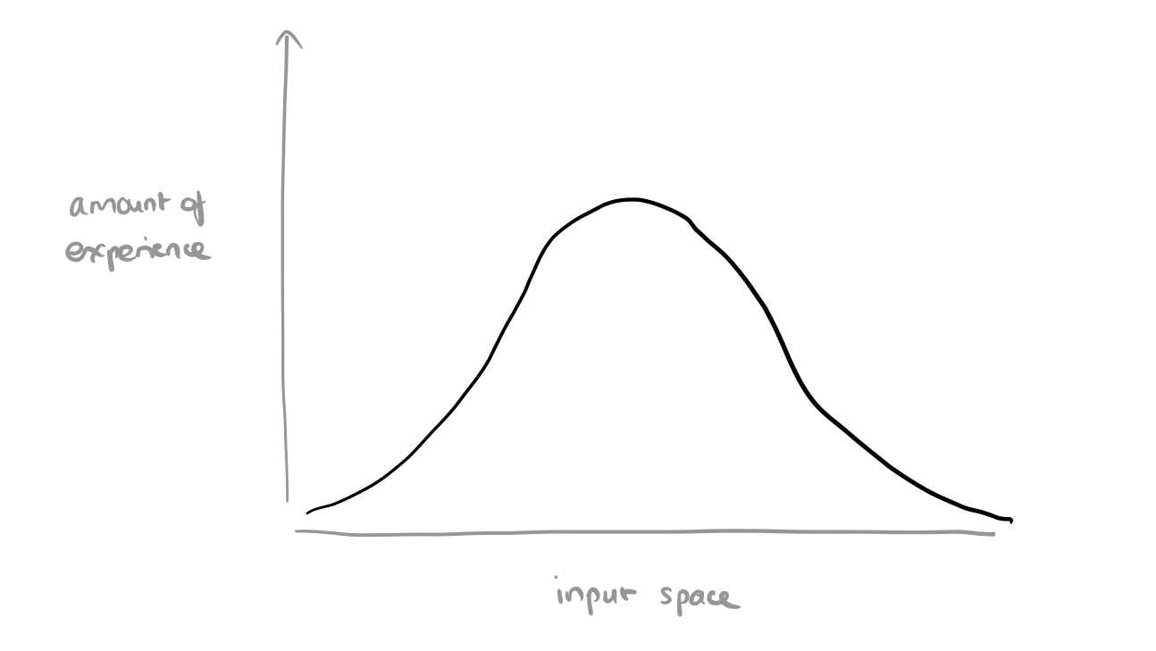
When we take a truncated normal at sampling time, we’re basically restricting inputs to the parts where the model has more experience. The more restrictive the truncation (narrower the selection), the higher we’d expect the quality of the generated samples to be. When we loosen the restriction by widening the selection the overall quality goes down, but we get more diversity.
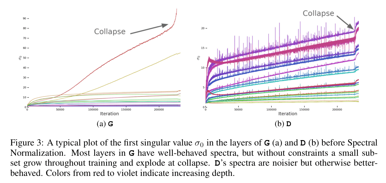
Instability
Section 4 of the paper probes the causes of instability in training. At the point of training collapse, the spectral norm in the generator network explodes.
Controlling for this on its own isn’t enough to induce stability though. Enforcing stability requires the generator and discriminator working hand-in-hand with strong constraints in the discriminator. However, these incur a dramatic cost in performance. In the end, best results were obtained by allowing collapse to occur during the later stages of training, by which time the model is sufficiently trained to achieve good results.
Bigger datasets
In addition to ImageNet, LS-GAN is also trained on the the 8.5K most common labels of the JFT-300M dataset (some 292M images, two orders of magnitude bigger than ImageNet). For this dataset further extending the capacity of the base channels proved beneficial.
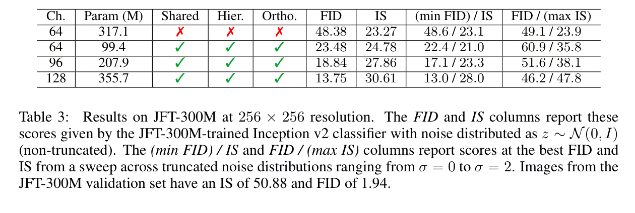
Interestingly, unlike models trained on ImageNet, where training tends to collapse without heavy regularization, the models trained on JFT-300M remain stable over many hundreds of thousands of iterations. This suggests that moving beyond ImageNet to larger datasets may partially alleviate GAN stability issues.
