Uncertainty propagation in data processing systems Manousakis et al., SoCC’18
When I’m writing an edition of The Morning Paper, I often imagine a conversation with a hypothetical reader sat in a coffee shop somewhere at the start of their day. There are three levels of takeaway from today’s paper choice:
- If you’re downing a quick espresso, then it’s good to know that uncertainty can creep into our data in lots of different ways, and if you compute with those uncertain values as if they were precise, errors can compound quickly leading to incorrect results or false confidence.
- If you’re savouring a cortado, then you might also want to dip into the techniques we can use to propagate uncertainty through a computation.
- If you’re lingering over a latte, then the UP (Uncertainty Propagation) framework additionally shows how to integrate these techniques into a dataflow framework.
We implement this framework in a system called UP-MapReduce, and use it to modify ten applications, including AI/ML, image processing, and trend analysis applications to process uncertain data. Our evaluation shows that UP-MapReduce propagates uncertainties with high accuracy and, in many cases, low performance overheads.
Are you sure?
Uncertainty can arise from a number of different sources including probabilistic modelling, machine learning, approximate computing, imprecise sensor data, and such like.
For many applications, uncertain data should be represented as probability distributions or estimated values with error bounds rather than exact values. Failure to properly account for this uncertainty may lead to incorrect results. For example, Bornholt et al. have shown that computing speeds from recorded GPS positions can lead to absurd values (e.g., walking speeds above 30mph) when ignoring uncertainties in the recordings.
If you have a dataflow system with computation based on a DAG, then uncertainty in upstream data values needs to flow through the computation. For example, consider a simple 2-node DAG where an approximate query is used to produce an approximate count of the number of customers in different age groups (e.g., using BlinkDB), and then we take a weighted average of those groups.
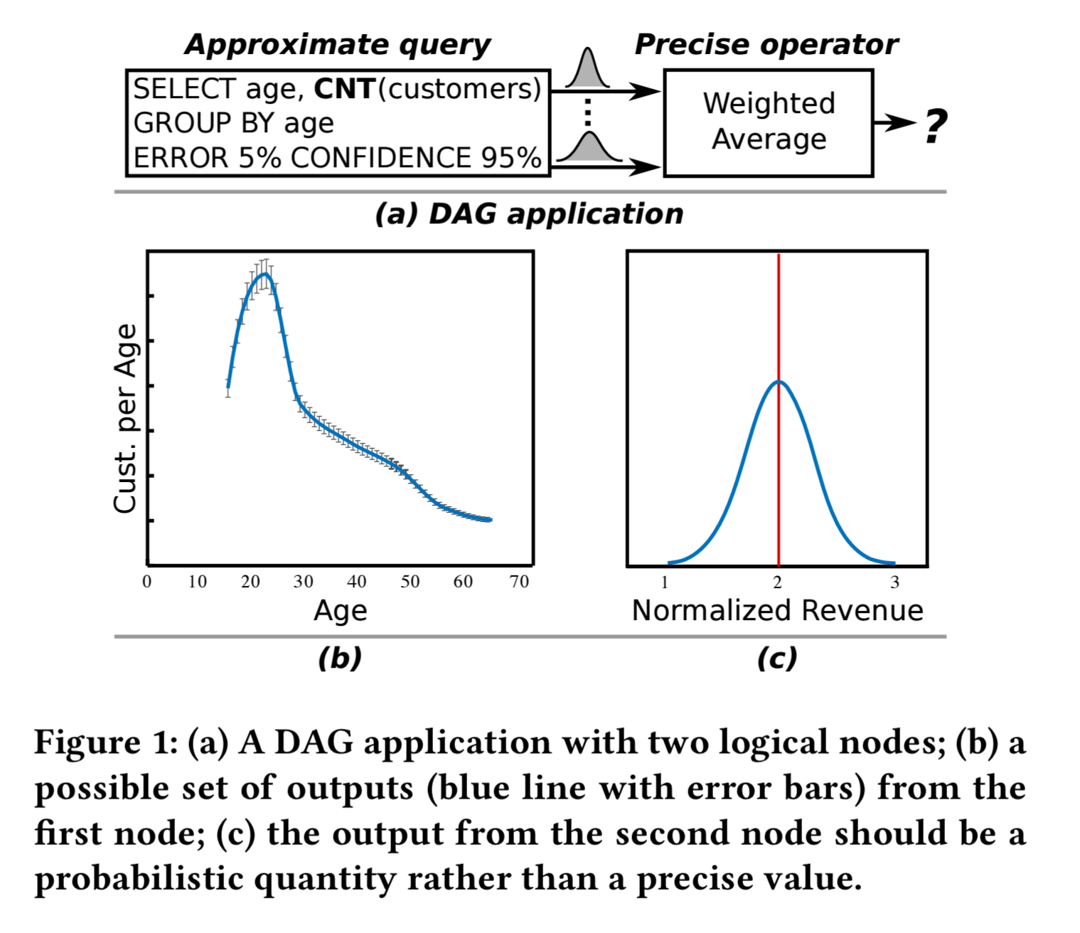
The second node will by default produce a single value, but in reality it should result in a distribution. There may be meaningful parts of that distribution where the outcome would be disadvantageous (for example), but the probability of this is completely lost when reporting a single value.
Uncertainty propagation
Our method offers, to the best of our knowledge, the only known computationally tractable (and as our evaluation will show, potentially with low overheads) large-scale uncertainty propagation.
Consider a function , where
is an arbitrary function without side-effects representing the computation at a node in a dataflow,
is a set of random variables representing inputs with uncertainties, and
is a set of random variables representing outputs with uncertainties. Depending on the nature of
, we can use different statistical methods to approximate the mean and variance of each variable in the output.
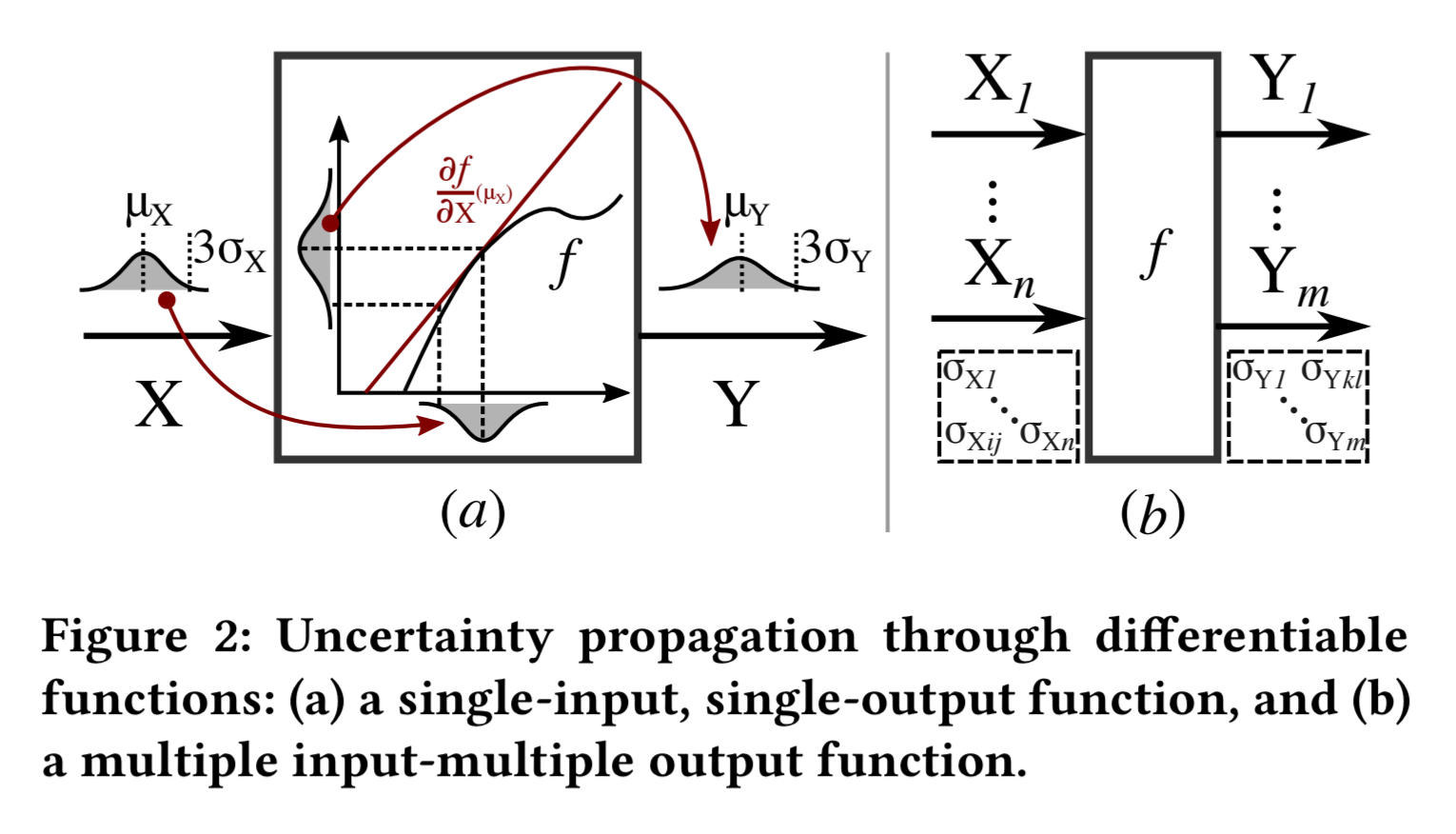
When is a continuous differentiable function we can use first-order Differential Analysis:
The general strategy is to compute
by approximating
using its first-order Taylor series at the expected value of
. This approximation is accurate if
is roughly linear around the support (in other words, neighborhood) of
…
When there are multiple inputs and multiple outputs, the calculation also needs to take into account the covariances between the outputs.
When is a semi-continuous function we have two possibilities. If the support of each input mostly or entirely falls within a continuous differentiable part of the function then we can use Differential Analysis (DA) as before. If it spans a discontinuity then we have to use Monte Carlo simulation. For example, consider the function
when
, and
otherwise. If each input is greater than
then we can use DA.
We use Monte Carlo simulation to approximate
for functions
that do not meet (or the developers do not know whether they meet) the requirements for DA.
is evaluated on
randomly drawn samples of the input, and the outputs are used as an approximation of
.
To generate accurate samples, one must know the joint density of
and pay the heavy computational cost of any rejection-sampling algorithm. Unfortunately that cost grows exponentially with an increasing size of
and thus we resort to two approximations:
- Given input distributions, generate samples accordingly and ignore covariances
- In the absence of full distributional information, assume that each input is normally distributed with the same mean and covariance matrix as the unknown distribution. (This approximation works because the mean and variance estimation of Y depends solely on the mean and variance of
).
Uncertainty propagation in dataflows
As stated earlier, in a dataflow graph we need to perform uncertainty propagation at all nodes downstream of uncertain data. For Monte Carlo simulation-based uncertainty propagation (UP-MC) we can just treat a node as a black box, dynamically generate samples from the input set, and compute the mean and variance for each output using empirically derived distributions (or assume normal distributions in the absence of this information).
The implementation of Differential Analysis (henceforth called UP-DA) is more challenging. Specifically, when a DAG node produces multiple outputs, we view it as being implemented by multiple sub-functions, each producing one of the outputs… input covariances can require additional data flow to be added to the DAG for computing output variances and covariances.
If the programmer can provide a partial derivative function, then using this often gives better performance than resorting to numerical differentiation.
Observe that we might make a saving early in the dataflow by introducing uncertainty (e.g. by computing an approximate result), but then we have to pay more later for the resulting uncertainty propagation. The evaluation explores this trade-off.
UP-MapReduce is an implementation of the above ideas in the in MapReduce.
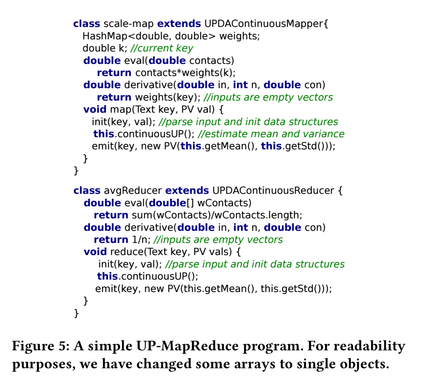
The UP-MapReduce extension includes three Mapper and three Reducer classes that implement UP-MC, UP-DA for continuous functions, and UP-DA for semi-continuous functions. The extension also introduce the uncertain type PV (Probabilistic Value) which contains one or more random variables, each described by a mean, a variance-covariance matrix, and possibly an entire empirical distribution.
The UP-DA Continuous Reducer class for example provides an abstract derivative method that a developer can implement to provide a closed-form derivative function.
Uncertainty propagation in practice
We have built a toolbox of common operations (e.g., sum) and modified ten common data processing applications using UP-MapReduce to process uncertain data.
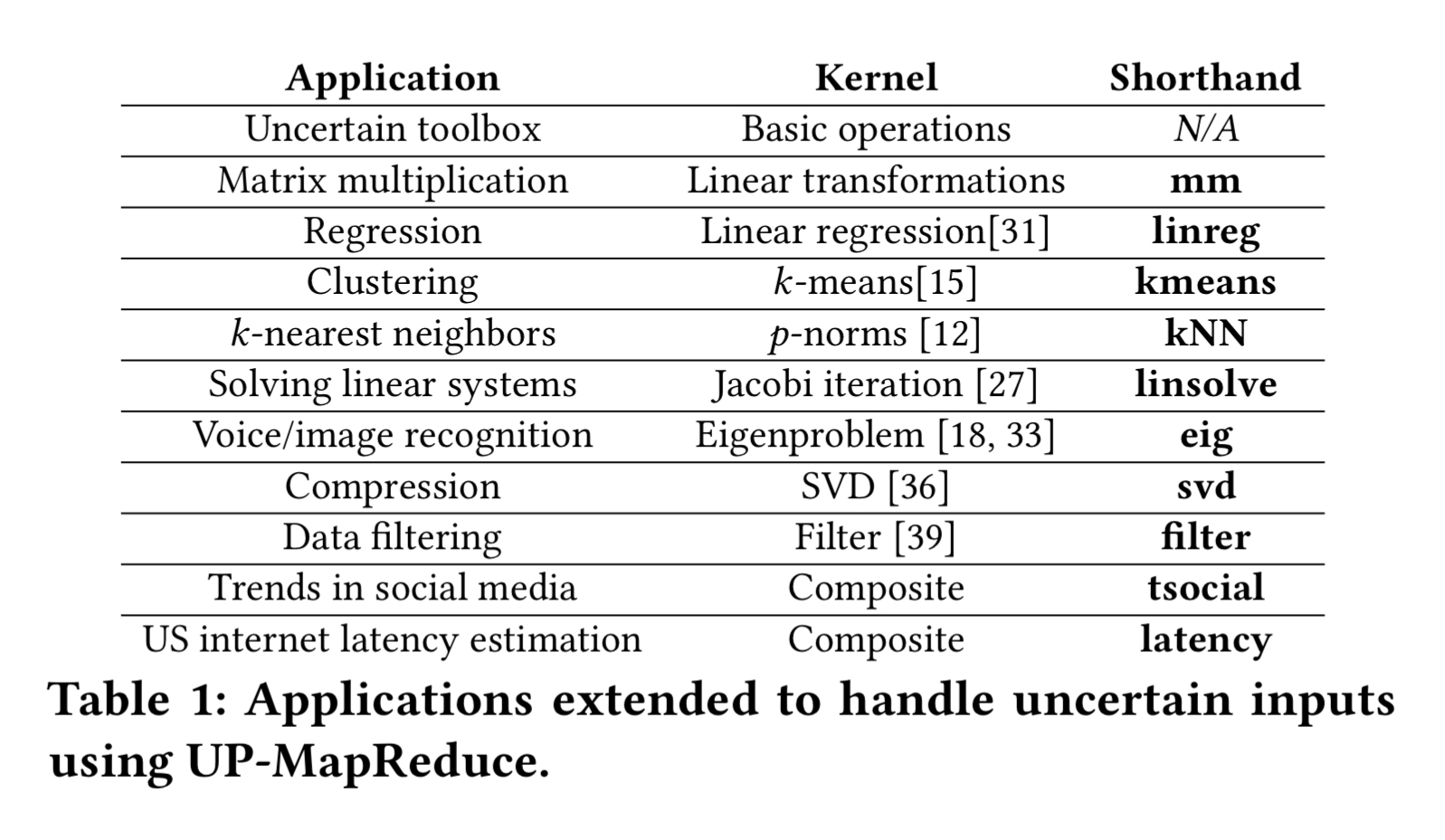
Baselines for the evaluation are established by running a large Monte Carlo experiment over a precise version of each application.
When input errors are small (e.g. below 3%) then UP-MapReduce estimates means with very low error.
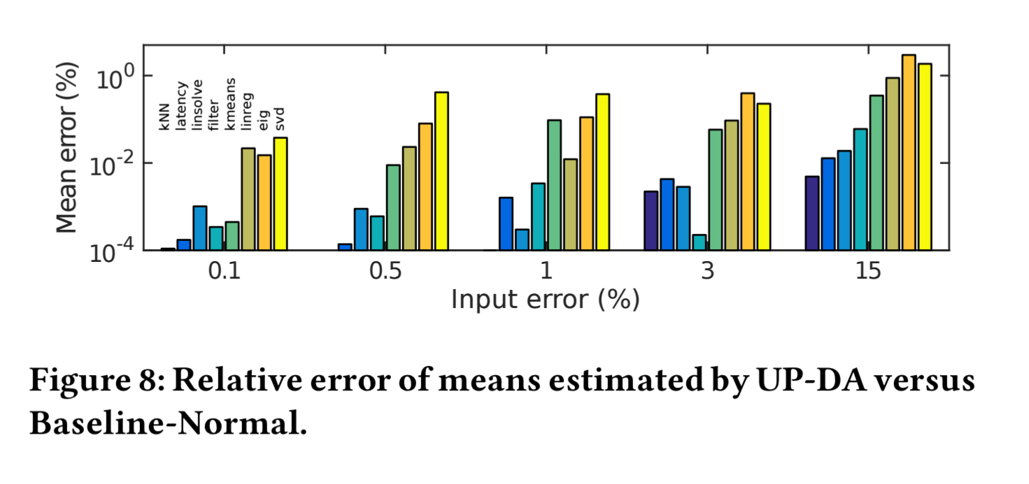
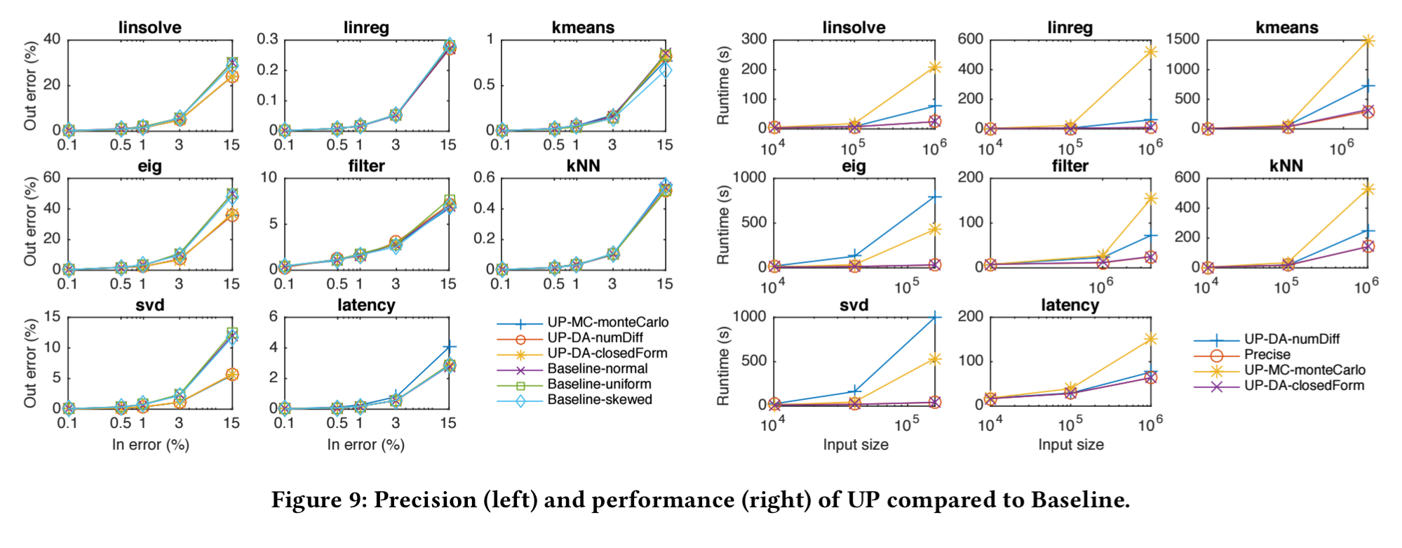
The following figure shows the relative errors and execution times for the three variants of UP-MC as compared to the baseline.
For six of the applications UP-MapReduce is highly accurate, but when input errors are significant (e.g. eig, svd) its estimated relative errors can deviate noticeably from baseline values. The best performance is obtained when using closed-form (user provided) derivatives.
tsocial and latency are both multi-stage approximate workflows. The following chart shows the execution times and maximum relative errors for sampling rates from 0.1% to 100% (precise).
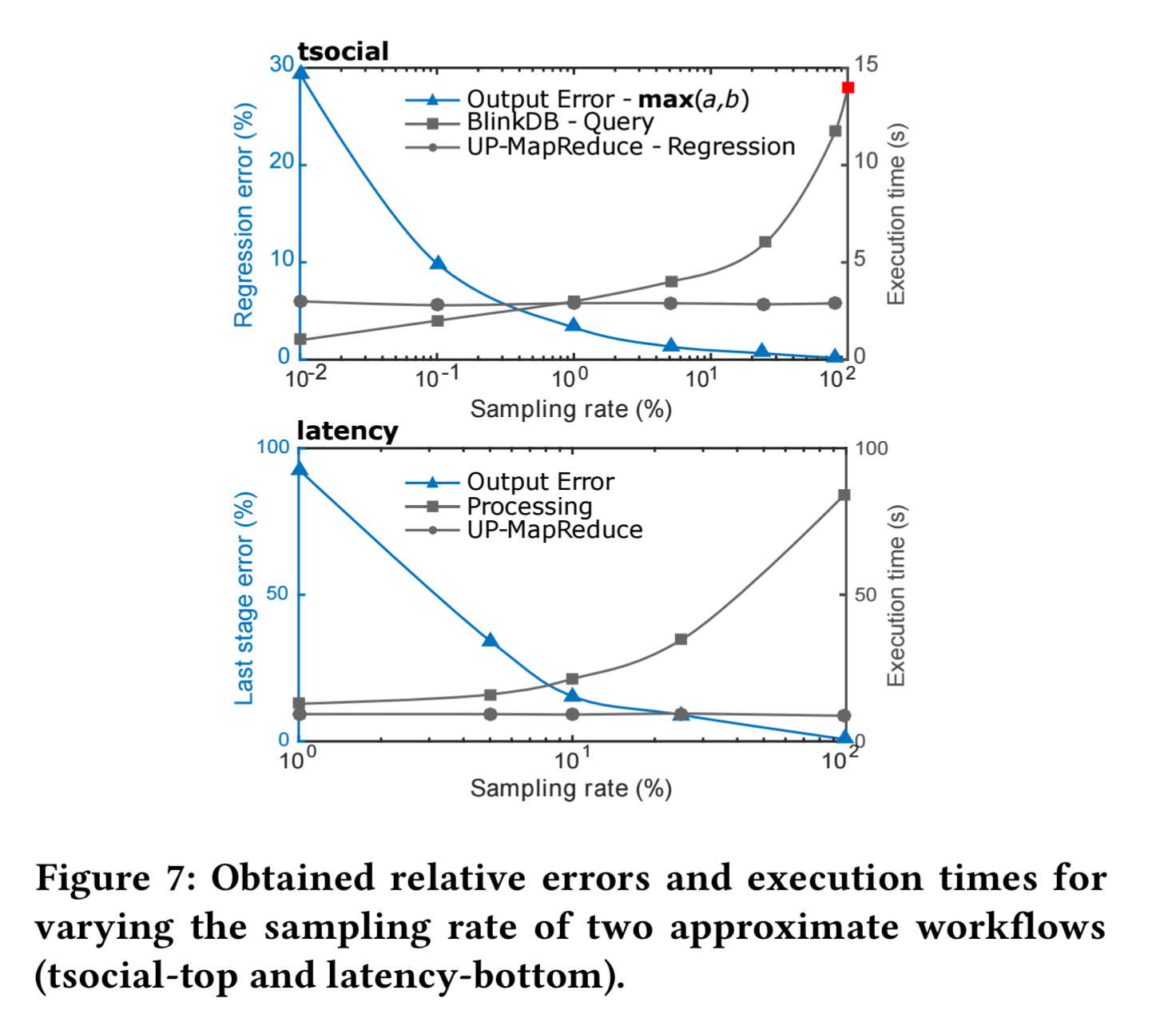
For tsocial, a sampling rate of 80% or less is required before the overheads of uncertainty propagation are outweighed by the sampling benefits.
Experimentation with ten common data analytic applications revealed that UP-MapReduce is highly accurate in many cases, while its performance overheads are very low— an average of 6% performance degradation— when closed-form derivatives are provided. When numerical differentiation or Monte Carlo simulation must be used, overheads can become much more significant as input size increases. Fortunately, the impact of these overheads on overall execution time can be reduced by allocating additional computational resources.
