STTR: A system for tracking all vehicles all the time at the edge of the network Xu et al., DEBS’18

With apologies for only bringing you two paper write-ups this week: we moved house, which turns out to be not at all conducive to quiet study of research papers!

Today’s smart camera surveillance systems are largely alert based, which gives two main modes of operation: either you know in advance the vehicles of interest so that you can detect them in real time, or you have to trawl through lots of camera footage post-facto (expensive and time-consuming). STTR is a system designed to track all of the vehicles all of the time, and store their trajectories for ever. I certainly have mixed feelings about the kinds of state surveillance and privacy invasions that enables (it’s trivial to link back to individuals given trajectories over time), but here we’ll just focus on the technology. Since the system is design with pluggable detection and matching algorithms, then given some calculations around volume it ought to be possible to use it to track objects other than vehicles. People for example?

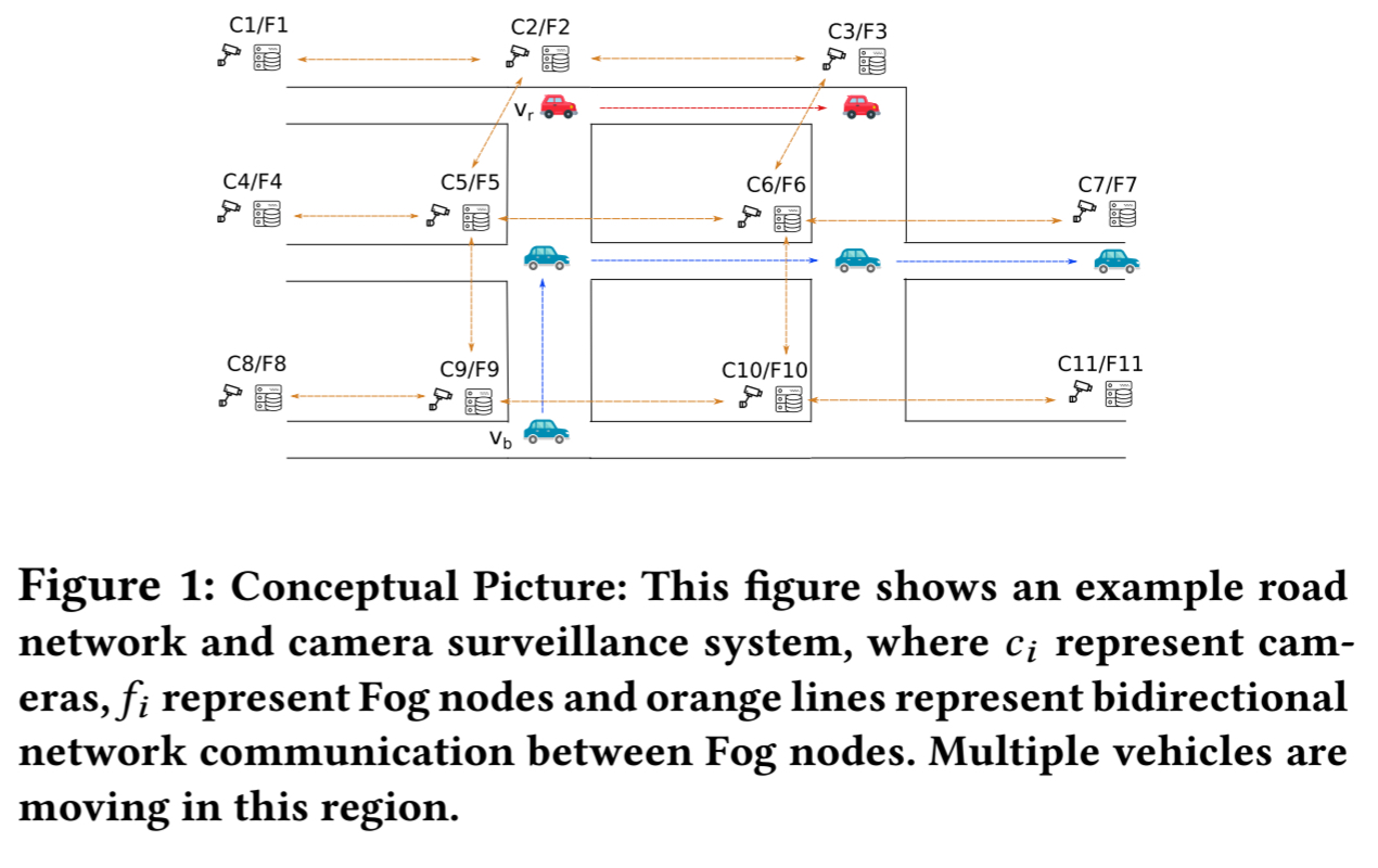
Assuming the availability of suitable detection and matching (figuring out if a vehicle is one you have seen before) algorithms, then the biggest challenge involved in tracking all of the vehicles all of the time is managing network bandwidth and storage. Storing and sending raw video clearly doesn’t work, so STTR simply stores vehicle trajectories (presumably some window, e.g. 24 hours, of video could also be accommodated) and processes video at local nodes. An edge/fog node can have multiple connected cameras.

Processing sensor streams (especially cameras) at the edge of the network is advantageous for three reasons: (a) reducing the latency for processing the streams, (b) reducing the backhaul bandwidth needed to send raw sensor streams to the cloud; and (c) preserving privacy concerns for the collected sensor data.

(I know what they mean by (c), even though the literal interpretation says the opposite of what the authors intended!).

Even when we’re storing only trajectories and processing video locally, all trajectories for all vehicles for all time still sounds like a lot of storage, and worse, potentially unbounded. The first key insight is that there is a pragmatic bound if we make some assumptions about vehicle density and vehicle lifetime (e.g. age of vehicle or miles travelled). The second key insight is that any one node only needs to manage data for a finite ‘activity region’ (loosely, the area that it covers before other cameras take over).

The finite size of the camera’s activity region gives us a very good property, because at any given time, the number of vehicles that are active under this camera has to be finite, for vehicles need to occupy space. Meanwhile, each vehicle’s life is also finite which indicates there exists trajectory upper bound for a given camera. Putting these facts together, we have the following simple idea – at any point in time, each camera stores the trajectory of vehicles that are active under its region.

A back of the envelope calculation with 5 cameras every mile, up to 100 simultaneously active vehicles for a given camera, and a vehicle lifetime of 150,000 miles, gives a storage requirement of around 1.1GB per camera.

Storing trajectories

The basic idea is to store the trajectory for a given vehicle at the node (camera) where it was last detected (active). Considering the following figure, the red car first seen at intersection by camera attached to fog node begins with a trajectory . When it moves through intersection we append to its known trajectory and migrate the record to node . When the vehicle then arrives at intersection we migrate the record once more, this time to node . The final trajectory record is .

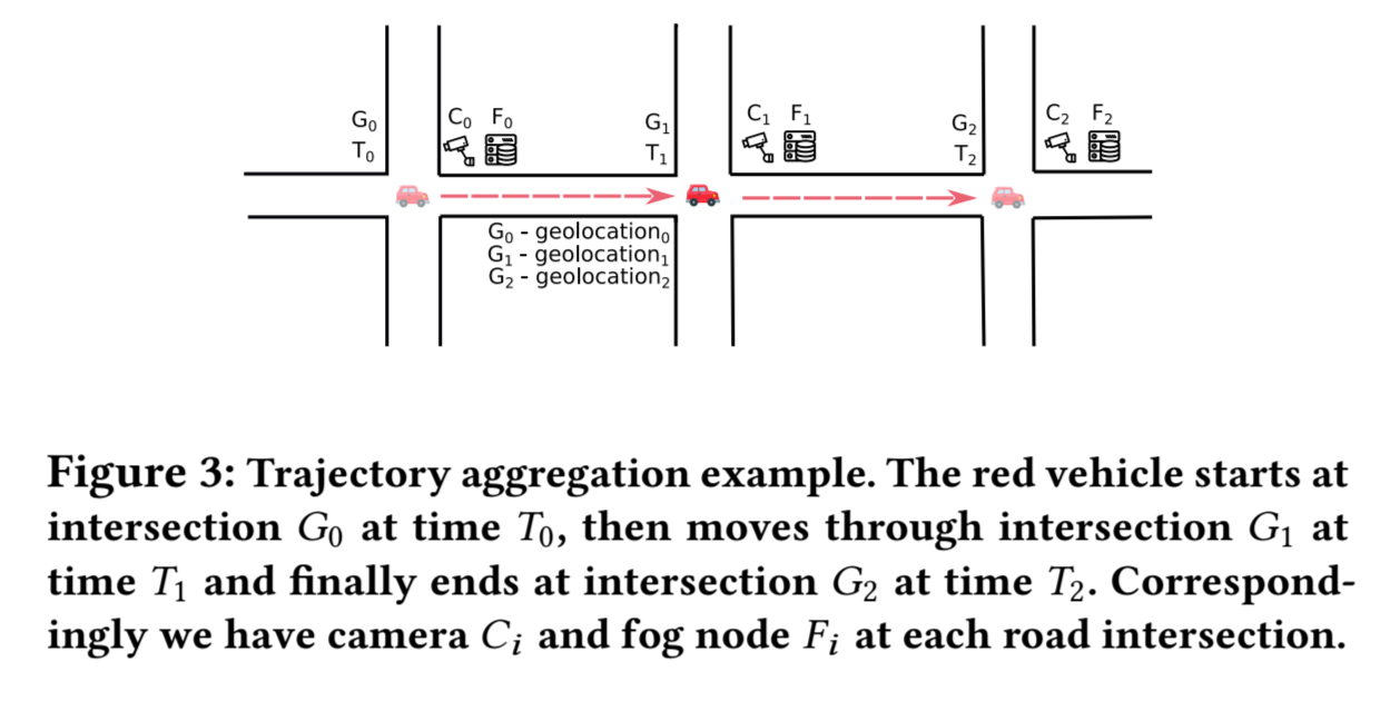
It’s easy to spot that as vehicle trajectories get longer over time, this process will result in a lot of network traffic to migrate trajectories from node to node. So instead of full trajectory migration, trajectories are partitioned across nodes and only aggregated once a node comes under storage pressure. (The current paper doesn’t consider querying, so implications for query efficiency here are unaddressed). We end with a lazy version of the basic algorithm.

Given the same vehicle movements as above the lazy trajectory aggregation might play out as follows:

• At time we create trajectory record (vertex) at node .
• At time we create an a trajectory vertex at node containing just the single step: , and we also create an edge from the vertex at to the newly created vertex at (so we’re building up a distributed graph structure).
• This process repeats when the vehicle arrives at , such that we end up with three linked trajectory portions.
• If node later comes under storage pressure we can aggregate its portion of the trajectory into the node at , ending up with an edge from directly to , and a trajectory vertex at of .

Once a vehicle is assumed to have reached end-of-life, its trajectory can be migrated to cloud storage or similar.

Network communication via forward and backward propagation

Information about detected vehicles is propagated through the network in order to build up the distributed graph and to reduce resource requirements at nodes. The primary mechanism is forward propagation. Once a vehicle has been detected by a camera, the vehicle’s signature (produced by an algorithm provided by domain experts) is sent to all cameras that are likely candidates for the vehicles to pass next. I infer that along with this message is sent the identifiers of all cameras in the propagation set. The cameras are then already primed to run the re-identification procedure when the vehicle is sighted. If a camera does detect a vehicle with a signature it received via forward propagation then it sends a sighting confirmation to all the other cameras in the propagation set, who can now drop it from their forward propagation local storage.

Sometimes a camera might detect a vehicle that it has not been primed to expect via forward propagation. In this case, backward propagation is used to send a message to candidate upstream cameras given the direction of travel. If such a camera cannot immediately re-identify the detected object in the backward propagation message it can simply discard it.

System architecture

The overall architecture of the STTR system looks like this:

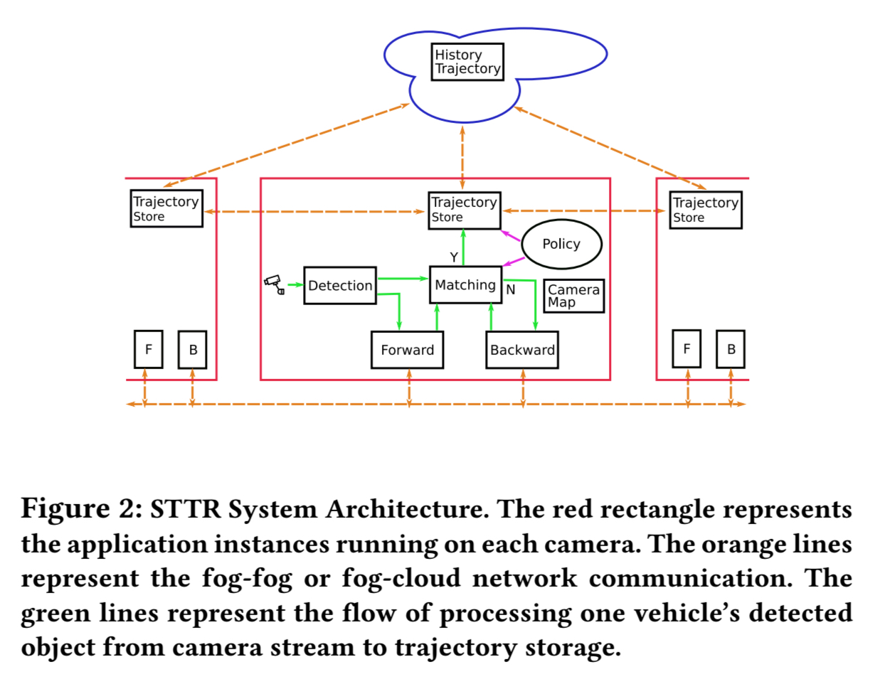
Each fog node runs a collection of seven modules per camera (e.g., in a container).

• The detection module takes as input a raw video stream from the camera, and outputs a stream of detected object (signatures).
• The matching module implements the re-identification algorithm, looking for a match with a detected object in the candidate vehicle pool assembled from forward propagation messages
• The camera map module maintains the geographical relationship between cameras
• The forward and backward modules implement forward and backward propagation
• The trajectory store manages trajectories as previously discussed and optimises network consumption
• The policy module supports system configuration

The evaluation implementation is written in Python using ZeroMQ for communication between nodes and Redis as a persistent store.

Evaluation

The evaluation is based on a simulation using the SUMO road traffic simulation package with a 10,000 second traffic flow emulation. Traffic is generated using a probability-based model. The fog computing topology is emulated using MaxiNet. The focus of the experiments is on understanding the storage and network bounds, and the impact of latency in forward and backward propagation. The short summary is that things pretty much work as you would expect. For example, if you have lower camera density then each camera uses more storage (since it is covering a larger area). The critical factor for enabling real-time surveillance turns out to be the speed of the re-identification algorithm.

Plans for future work include:

• Creation of efficient spatial and temporal index structures to support querying the network
• Improving confidence in the calculated trajectories using a probabilistic approach to trajectory generation and maintenance
• An on-campus deployment in conjunction with the campus police department