Debugging with intelligence via probabilistic inference Xu et al., ICSE’18
Xu et al. have built a automated debugger that can take a single failing test execution, and with minimal interaction from a human, pinpoint the root cause of the failure. What I find really exciting about it, is that instead of brute force there’s a certain encoded intelligence in the way the analysis is undertaken which feels very natural. The first IDE / editor to integrate a tool like this wins!
The authors don’t give a name to their tool in the paper, which is going to make it awkward to refer to during this write-up. So I shall henceforth refer to it as the PI Debugger. PI here stands for probabilistic inference.
We model debugging as a probabilistic inference problem, in which the likelihood of each executed statement instance and variable being correct/faulty is modeled by a random variable. Human knowledge, human-like reasoning rules and program semantics are modeled as conditional probability distributions, also called probabilistic constraints. Solving these constraints identifies the most likely faulty statements.
In the evaluation, when debugging problems in large projects, it took on average just 3 interactions with a developer to find the root cause. Analysis times are within a few seconds. One of the neat things to fall out from using probabilistic inference is that the developer interacting with the system doesn’t have to give perfect inputs – the system copes naturally with uncertainty.
Intuition
To see how PI Debugger uses probabilistic inference to pinpoint likely root causes, let’s work through a concrete example. Here’s a Python program defining a function path_url. The function takes an input url and safely encodes the path portion. For example, given as input https://example.com/abc def?x=5 the output should be https://example.com/abc%20def?x=5.
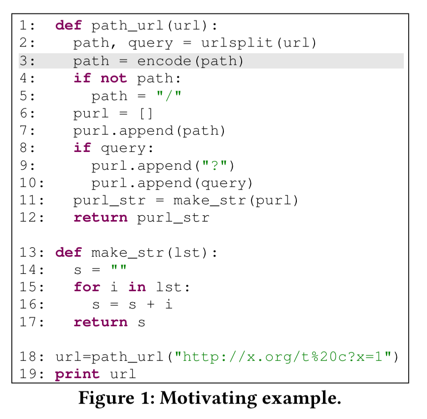
This program has a bug. When given an already encoded input, it encodes it again (replacing % with ‘%25’). For example, the input https://example.com/t%20c?x=1 results in the output https://example.com/t%2520c?x=1, whereas in fact the output should be the same as the input in this case.
Let’s put our probabilistic thinking caps on and try and to debug the program. We ‘know’ that the url printed on line 19 is wrong, so we can assign low probability (0.05) to this value being correct. Likewise we ‘know’ that the input url on line 1 is correct, so we can assign high probability (0.95). (In probabilistic inference, it is standard not to use 0.0 or 1.0, but values close to them instead). Initially we’ll set the probability of every other program variable being set to 0.5, since we don’t know any better yet. If we can find a point in the program where the inputs are correct with relatively high probability, and the outputs are incorrect with relatively high probability, then that’s an interesting place!
Since url on line 19 has a low probability of being correct, this suggests that url on line 18, and purl_str at line 12 are also likely to be faulty. PI Debugger actually assigns these probabilities of being correct 0.0441 and 0.0832 respectively. Line 18 is a simple assignment statement, so if the chances of a bug here are fairly low. Now we trace the data flow. If purl_str at line 12 is likely to be faulty then s at line 16 is also likely to be faulty (probability 0.1176).
Line 16 gets executed three times, two of which produce correct outputs, and one of which produces incorrect outputs. This reduces the suspicion on line 16 itself (now probability 0.6902), and suggests the first instance of i at line 16 is faulty.
Using variable name similarity inference rules, PI Debugger assigns higher correlation probability between variables with similar names (e.g. path_url and url) than those with dissimilar names (e.g. url and make_str). If the first instance of i is faulty, then purl at line 7 is also likely faulty. This could be due to a faulty value of path or a bug in append. PI Debugger knows to assign lower probabilities to bugs in library code.
If path is faulty on line 7, then either path itself is faulty, or the output of line 3 is faulty. We know that the input url on line 1 is likely correct, so the odds are in favour of the rhs of the assignment on line 3 being the culprit. And indeed it is – we should have a test to make sure that path is not already encoded before we call encode.
Although we describe the procedure step-by-step, our tool encodes everything as prior probabilities and probabilistic constraints that are automatically resolved. In other words, the entire aforementioned procedure is conducted internally by our tool and invisible to the developer.
PI Debugger overview
PI Debugger encodes the process just described, and consists of four main components: the tracing component, the probabilistic constraint encoding component, the probabilistic inference engine, and the feedback component.
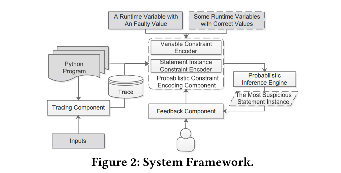
The inference procedure can be intuitively considered as a process of fusing hints from various observations (i.e., High/Low prior probabilities) through the propagation channels dictated by the constraints.
Before beginning the analysis all the runtime variables in the program trace are converted in static single assignment (SSA) form. We then proceed in two main phases:
- Inferring variable correctness probabilities. This step uses dynamic slicing and propagation constraint probabilities. For example, given an assignment
a = b + c, then if any two of the three components are correct, we can infer that the other is also likely to be correct. The encodings are sent to the inference engine which builds a factor graph and computes posterior probabilities using the Sum-Product algorithm. - Inferring statement instance correctness. This stage combines the probabilities from the first stage with domain knowledge rules to determine the probability of each executed statement being correct. There are three types of generated constraints (i) constraints correlating variable probabilities and statement instance probabilities, (ii) constraints from program structure, for example a function with a large number of statements is more likely to include the faulty statement, (iii) constraints from naming convention, on the assuming that function and variable names suggest functionality to some extent. These constraints and prior probabilities are once more sent to the inference engine.
We compute marginal probabilities based on the Sum-Product algorithm. The algorithm is essentially a procedure of message passing (also called belief propagation), in which probabilities are only propagated between adjacent nodes. In a message passing round, each node first updates its probability by integrating all the messages it receives and then sends the updated probability to its downstream receivers. The algorithm is iterative and terminates when the probabilities of all nodes converge. Our implementation is based upon libDAI, a widely used open-source probabilistic graphical model library.
At the end of the process, the most probable root cause is reported to the developer. If the developer disagrees, they can provide their assessment of the likelihood the operands in the reported statement are faulty. This then becomes a new observation and we can run inference again.
Constraint generation
Section 5 in the paper contains detailed information on the constraint generation process. For variables there are three encoding rules, covering the forward causality of a statement (e.g. the likelihood of the lhs of an assignment being correct given the rhs), the backward causality (e.g. the likelihood of the rhs of an assignment being correct given the lhs), and causality for control predicates (the likelihood of the correct branch being taken). The computation rules propagate probability differently depending on the type of statement involved (e.g., assignment, mod, attribute read, read of a collection element, equivalence,…).
Three different kinds of constraints are generated for statement instances:
- value-to-value statement constraints model the causality between variable probabilities and statement instance probabilities
- program structure constraints modelling hints from program structure, and
- naming convention constraints modelling hints from names.
Evaluation results
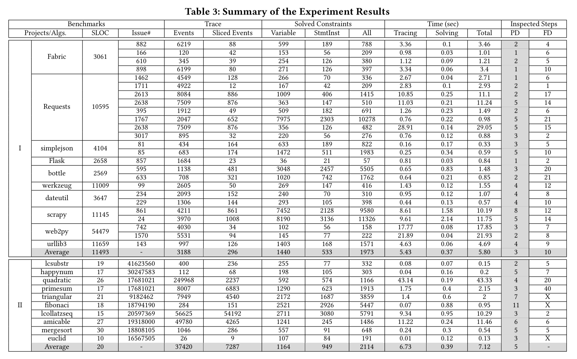
PI Debugger is applied to a set of real world bugs taken from some of the largest Python projects on GitHub. The monster table below summarises the results. The ‘PD’ column reports the number of interactions, including the final root cause step. (The ‘FD’ column is the number of steps taken by the Microbat debugging tool). PI Debugger completes inferences in around a second for most cases.
(Enlarge)
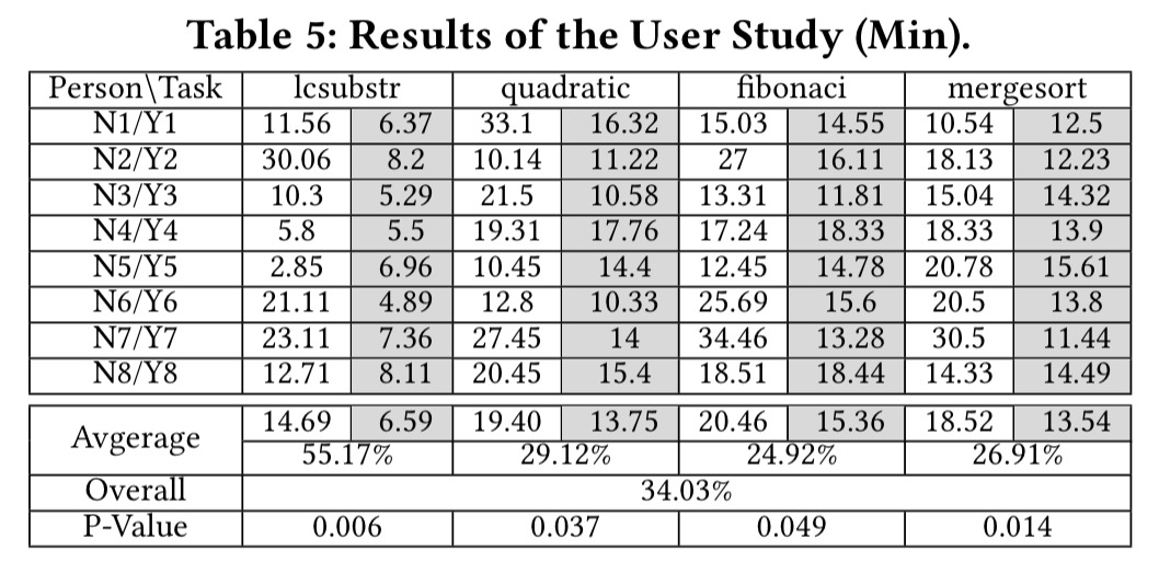
Four bugs are further selected for a user study:
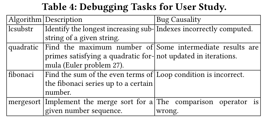
16 students are randomly partitioned into two groups and asked to find the root cause of the bugs, one group using PI Debugger, and the other using pdb. On average, the PI Debugger group were 34% faster.
The results show that our technique can identify root causes of a set of real-world bugs in a few steps, much faster than a recent proposal that does not encode human intelligence. It also substantially improves human productivity.

“For example, given an assignment a = b + c, then if any two of the three components are correct, we can infer that the other is also likely to be correct.”
I’m not convinced by this: what about the arithmetic overflow case? b and c would be correct, but a might not be. (I’m fairly sure this can be accounted for in implications derived from the ‘+’ operator.) In general, discontinuities in behaviour may provide some rather tricky inferences of correctness probabilities. But I suppose knowing the actual values of the variables in the failing case could be used to simplify this.
I would suggest πDebug as a name.
The beauty of the probabilistic approach is that it’s only assigning a likelihood, so if it turns out this assumption is wrong, it should in theory get overturned eventually. The authors rely on this for contributions from humans that may make wrong judgements, but I guess the same logic applies to ‘+’ as well :).