WSMeter: A performance evaluation methodology for Google’s production warehouse-scale computers Lee et al., ASPLOS’18

(The link above is to the ACM Digital Library, if you don’t have membership you should still be able to access the paper pdf by following the link from The Morning Paper blog post directly.)

How do you know how well your large kubernetes cluster / data centre / warehouse-scale computer (WSC) is performing? Is a particular change worth deploying? Can you quantify the ROI? To do that, you’re going to need some WSC-wide metric of performance. Not so easy! The WSC may be running thousands of distinct jobs all sharing the same underlying resources. Developing a load-testing benchmark workload to accurately model this is ‘practically impossible.’ Therefore, we need a method that lets us evaluate performance in a live production environment. Google’s answer is the Warehouse Scale performance Meter (WSMeter), “a methodology to efficiently and accurately evaluate a WSC’s performance using a live production environment.” At WSC scale, even small improvements can translate into considerable cost reductions. WSMeter’s low-risk, low-cost approach encourages more aggressive evaluation of potential new features.

Challenges in defining a WSC performance metric

Consider a change to rollout a new DVFS (power management) policy. Is the impact positive or negative? The answer is both, depending on your perspective!

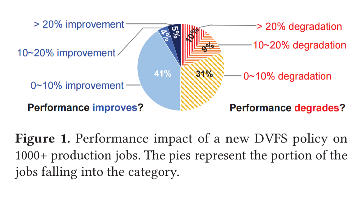
We observe that half of the jobs experience performance boost while the other half suffer from degradations. It is difficult to finalize the decision because the jobs have conflicting performance behaviors and there is no metric to summarize the overall performance impact.

Even when you pick one job with overall improvement performance, and one with overall degraded performance, and then look at the distribution across the instances of those jobs, it’s hard to draw clear conclusions given the input data variance and resource interference.

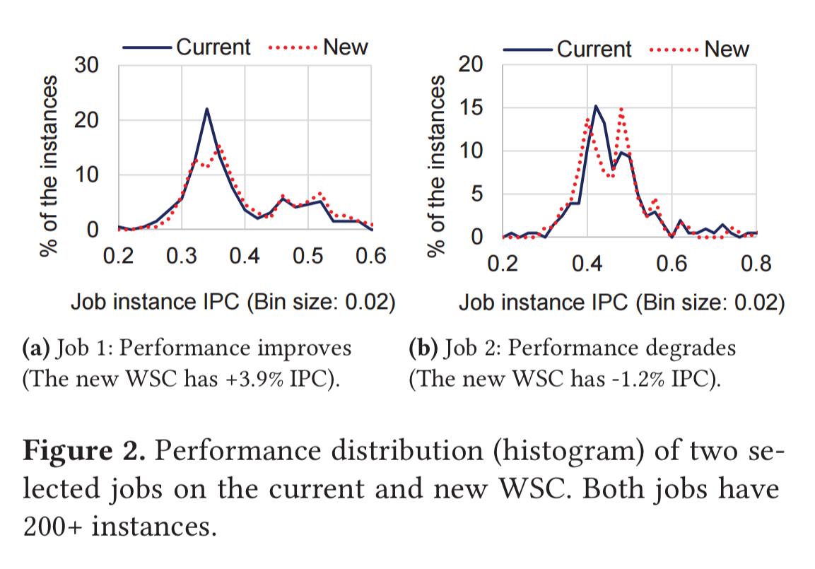
… the jobs and machines in WSCs show diverse behaviors at scale, making it difficult to accurately quantify the performance from few observations.

Quota-weighted performance

The goal is to boil the performance of the whole WSC down to a single number (we’ll talk about the limitations of that shortly, but for now let’s just roll with it). We can measure the performance of individual jobs, and intuitively the metric should be some aggregation of the per-job performance. Suppose the performance of an individual job i is given by , then the simplest measure would be to take the mean value of across all jobs. WSMeter starts there, but makes three tweaks:

1. It uses a weighted average, where the performance of a given job is weighted by a factor indicating its importance. For Google, the weighting factor is based on a job’s quota, specifically the CPU quota, indicating the maximum amount of CPU the job is allowed to use. The weighting factor for a given job is the CPU quota for that job, divided by the total quota across all jobs.
2. For the job performance metric, there are two choices. If all jobs in the scope of interest share the same user-level performance metric, then that can be used. Otherwise Google use Instructions per Cycle (IPC) as the performance metric. For Google jobs, this correlates well with user-level performance metrics.
3. Instead of using the performance of all jobs in the metric calculation, it uses only a subset of the jobs. An analysis of Google workloads shows that much of the CPU quota is consumed by a relatively smaller number of heavyweight jobs that are common across their WSCs. (See the charts below).

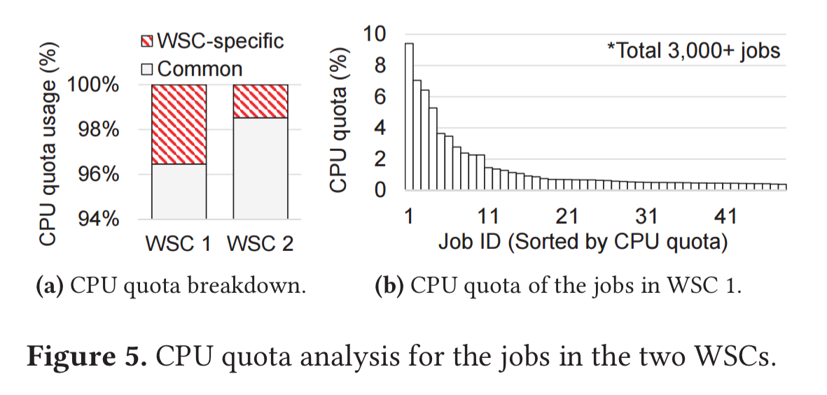
We find that many of these heavyweight jobs are basic infrastructure jobs (e.g., databases, caches, distributed locks) that the other higher-level jobs utilize; they are therefore common across WSCs…

WSMeter samples from the top-N common jobs, and find through empirical investigation that considering 10%-20% of the common jobs reduces the deviation from the results observed when considering all common jobs to just a few percent.

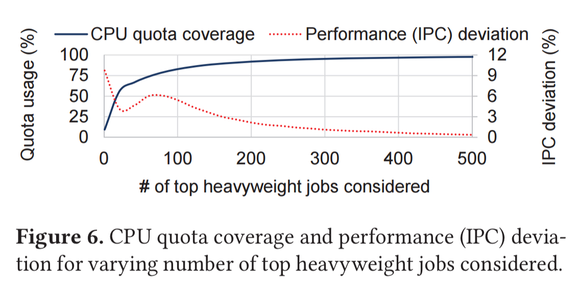
We emphasize that the heavyweight jobs are still much more diverse compared to the jobs in typical load-testing benchmark suites (e.g., about a dozen), highlighting the need for an evaluation using live environments.

The thing that jumps out to me here is that this is a rich-get-richer scheme. By boiling WSC performance down to a single number, and deploying upgrades based on their ability to improve that number, we end up improving the performance of the largest jobs by weight in the WSC. Of course, in aggregate that’s going to give the best overall improvement. But the metric allows all sorts of carnage to happen in the tail. (Think of the usefulness of e.g. mean latency vs 99th-%ile latency, or even seeing the full distribution). There are particular characteristics of Google’s workloads in their WSCs that make this trade-off work for them. It would be worth thinking about whether or not your own workloads share similar characteristics before rushing to use this single metric.

A statistical performance model

We have a metric, so now we can turn our attention to the best way to capture the underlying measurements in a production setting. There is natural performance variation across job instances (input parameters, neighbours, and so on), so we can’t rely on just a single measurement. Instead, we can treat the performance of a job as a random variable following a certain probability distribution.

The Central Limit Theorem then suggests that if we can make sufficient observations, we can accurately deduce the average statistic.

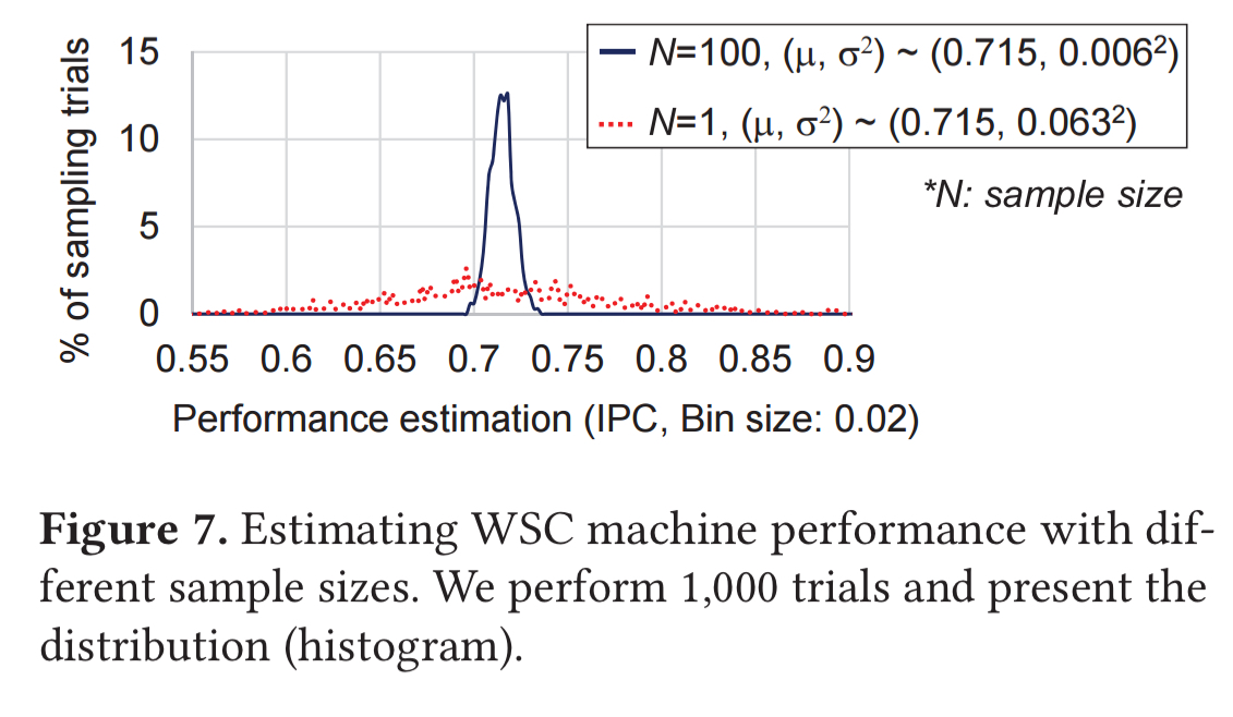
The following figure shows distribution of a sample’s mean for 1000 sampling trials using each of two different sample sizes. When N=100, you can see the estimations heavily clustered around the true value, while the sample with N=1 does not share this characteristic.

WSMeter estimates the performance of each selected job in this way, and using those job performance estimations as inputs to the quota-weighted averaging process we saw earlier. There’s a little bit of trickiness involved in summing the individual t-distribution random variables though:

As the summation of t-distribution random variables does not follow a t-distribution (or other well-known distributions), we approximate [the individual job performance metrics] to follow a normal distribution.

Under this assumption the weighted sum of per-job performance follows a normal distribution with mean and variance:

Empirical investigation shows that it is safe to ignore the covariance term (see section 4.3).

Therefore, we approximate the WSC performance as a normal random variable whose mean is the weighted sum of the per-job performance estimations and the variance is the weight-squared sum of the per-job variances (i.e., ignore the covariance term).

To control the accuracy of the result (i.e., the variance), we can adjust the number of observations for each job. Note that can be different for each job we want to sample. WSMeter gives this problem to a sat solver, asking it to find an optimal combination of s under the follow constraints:

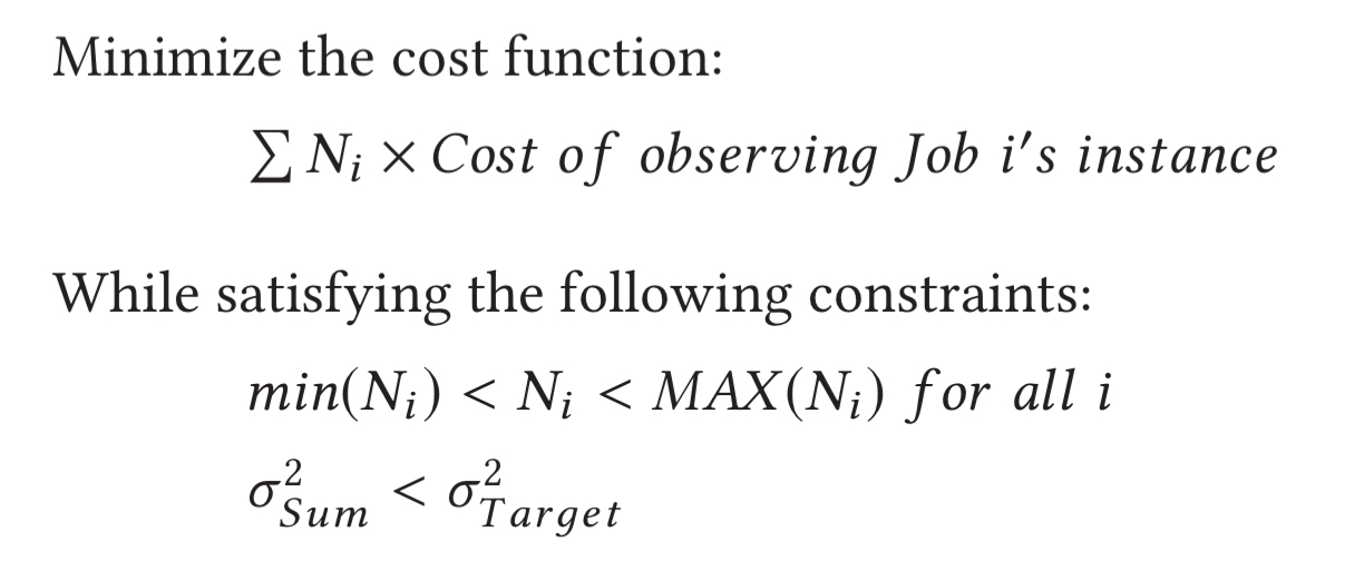
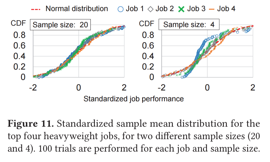
The minimum value of is set to 4, based on an analysis of the top four heavyweight jobs and the number of samples needed to ensure a normal distribution. This value is a trade-off balancing coverage, fidelity, and cost.

WSMeter in action

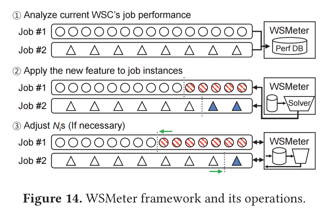
End-to-end, WSMeter looks like this:

(Enlarge)

Assessing a potential performance improvement is a five-step process:

1. The current WSC performance is baselined, using all the job instances in the WSC to calculate population performance statistics.
2. The jobs to be included in the target evaluation are selected to achieve the target weight-coverage. At this point it is also necessary to decide upon the desired evaluation fidelity.
3. The sat solver solves the optimisation problem to determine the number of job instances to observe for each job.
4. A testing cluster is built with the new feature. This can either be done by replacing existing machines in the WSC, or by adding new machines. The new job performance characteristics as well as the overall performance characteristics are then measured.
5. In the case that the new feature increases the performance variance of the jobs, the initial s may become insufficient. If so, the variances in the optimisation problem are updated and one more round of measurement is done until the requirement is satisfied.

For the case of a CPU upgrade, and a new DVFS policy…

… WSMeter accurately discerns 7% and 1% performance improvements from WSC upgrades using only 0.9% and 6.6% of the machines in the WSCs, respectively. We emphasize that naive statistical comparisons incur much higher evaluation costs (> 4x) and sometimes even fail to distinguish subtle differences.

The third case study is especially interesting, because it shows how the methodology can be applied to a WSC customer. A customer operates one compute-intensive service and one network intensive service of equal importance and cost, with 1,500+ instances of each job deployed on the cloud. The upgrade to be tested is a collection of compiler optimisations and software upgrades. When testing these changes in isolation, an 11% improvement is observed, but using WSMeter a picture of the real in-production gains, at around 6.6% emerges.

This discrepancy strongly encourages the WSC customers, service developers, and researchers, to evaluate new features on live WSCs to measure the realistic performance impacts.